6

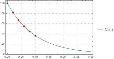
I'm trying to find an exponential model from data for a homework problem. There is an accompanying video explaining how to do the bigger problem but it omits any instructions on the step where the model is determined. Here is a screenshot of the video after the model is found:

enter image description here

I've attempted to follow the instructions in "The Student's Introduction to Mathematica" for using FindFit to determine such a model:

enter image description here

As you can see, the results don't match those in the video and there's some type of warning/error that I don't understand. I also attempted to use NonlinearModelFit with similar results.

Any help is greatly appreciated.

WXB13
  • 163
  • 2
  • 8
  • Sorry but I did search before asking this question as I always do. I tried a couple of different searches but I'm guessing that I didn't use the right combination of terms. I also try very hard to figure things out on my own and typically only resort to asking questions when I've hit a dead end. I know that there are probably a lot of people who try to get other people to do their homework but that is definitely not me. – WXB13 Sep 16 '14 at 09:05

3 Answers3

10

Exponents are always a headache for fitting. Fit the Log instead:

data = {{0, 100}, {.02, 81.87}, {.04, 67.03}, {0.06, 54.88}, {.08, 44.93}, {.1, 36.76}};
sol = FindFit[data /. {x_, y_} :> {x, Log@y}, la + t lb, {la, lb}, t];
{a, b} = Exp[{la, lb} /. sol];

(* {100.012, 0.0000451495} *)
Dr. belisarius
  • 115,881
  • 13
  • 203
  • 453
  • Employing the Log you can calculate the size of Borges' Library of Babel. See here: http://unendliches.net/english/index.htm?bbabel.htm – eldo Sep 16 '14 at 02:37
  • 1
    @eldo "En algún anaquel de algún hexágono (razonaron los hombres) debe existir un libro que sea la cifra y el compendio perfecto de todos los demás: algún bibliotecario lo ha recorrido y es análogo a un dios" – Dr. belisarius Sep 16 '14 at 02:55
  • 1
    "Yo siempre seré el futuro Nóbel. Debe ser una tradición escandinava." :) – eldo Sep 16 '14 at 03:06
  • I'm a relative newcomer to Mathematica and the class is a first year calc class so I'm having to figure out (i.e. "try" to figure out) some of the syntax and math concepts on the fly. By referencing the help system and executing bits and pieces of your code I've been able to figure out the ReplaceAll ("/.") and RuleDelayed (":>") operators that you're using. – WXB13 Sep 16 '14 at 05:16
  • I'm a little bit more fuzzy about the why/how of using Log and Exp in your answer. I'll try to explain my understanding (and lack thereof) and hopefully you'll be able to set me straight. Please forgive me if my questions are rather basic. I'm guessing that the transformation of (a*b)^t to la + t lb is done via applying Log to everything and the purpose of doing this is to get t out the exponent; in the last step Exp is applied to the results in order to reverse the Log applied in the previous step. – WXB13 Sep 16 '14 at 05:17
  • How close is my understanding of this? Why is the Log easier to fit?

    I'm still working on the Library of Babel problem. More updates to come...

    – WXB13 Sep 16 '14 at 05:18
  • 1
    @GaryWhite The Log is easier to fit because it is a straight line. There are numerical problems when fitting exponentials (the base of). You may help the algorithm by providing good hints: NonlinearModelFit[data, {a b^t, a > 0 && b > 0}, {{a, 100}, {b, 0.00005}}, t] – Dr. belisarius Sep 16 '14 at 05:45
9
data = {{0., 100.}, {0.02, 81.87}, {0.04, 67.03}, {0.06, 54.88}, {0.08, 44.93}, {0.1, 36.76}};

model = a Exp[-k t];

fit = FindFit[data, model, {a, k}, t]

{a -> 100.004, k -> 10.0033}

fun = Function[{t}, Evaluate[model /. fit]]

enter image description here

Plot[fun[t], {t, 0, 0.3},
 Epilog -> {PointSize[0.02], Red, Point[data]},
 PlotRange -> All,
 PlotTheme -> "Detailed"]

enter image description here

fun[0.2]

13.525

TableForm[Map[{#, Round[fun @ #, 0.01]} &, Range[0, 1, 0.1]],
 TableHeadings -> {None, {"t", "Q"}},
 TableDirections -> Row]

enter image description here

eldo
  • 67,911
  • 5
  • 60
  • 168
7

Check out the formula for capacitor discharge, it takes the form

chargeDecay=initialCharge Exp[- r/c t]

So

t = {0, 0.02, 0.04, 0.06, 0.08, .1}; 
q = {100, 81.87, 67.03, 54.88, 
 44.93, 36.76};
modelData = Transpose[{t, q}];
soln=FindFit[modelData, a Exp[-b x], {a, b}, x]
(*{a -> 100.004, b -> 10.0033}*)
Show[ListPlot[modelData, PlotStyle -> Red], 
Plot[a Exp[-b x] /. soln, {x, 0, 0.1}]]

Mathematica graphics

You can also use the following function which also provides more information.

nlm = NonlinearModelFit[modelData, a Exp[-b x], {a, b}, x]
nlm["AdjustedRSquared"]
(*1*)
nlm["ParameterTable"]
Zviovich
  • 9,308
  • 1
  • 30
  • 52
  • It's the same thing he's fitting Exp[-10.0033] == 0.000045:) – Dr. belisarius Sep 16 '14 at 01:09
  • Thanks for pointing me to NonlinearModelFit:) – eldo Sep 16 '14 at 01:57
  • Interesting; I was wondering where their formula came from and it never dawned on me to search for the formula for capacitor discharge (D'oh!). Does the negative sign reflect the fact that it's a discharge? – WXB13 Sep 16 '14 at 09:17
  • Dear @GaryWhite, indeed the negative sign makes the function's limit to infinite reach zero. Assuming[a > 0 && b > 0, Limit[ a Exp[-b t], t -> [Infinity]]] – Zviovich Sep 16 '14 at 12:48