I'd like to ask you if you see any difference between the two following ways of estimating parameters. Given my system of ordinary differential equations that I want to use to find the values of all the dependent variables through time, I have 2 options to find the parameters k1, k2, k3 to some curves. I describe these two after describing the example.
The problem
I want to fit k1, k2 and k3. In this example, I have 3 sets of data pertaining to the concentrations of A, B and X. This example was sent to me by someone who had taken it from the wolfram knowledge-base (in here.
Given a simple reaction A + 2B -> products, whereby two sub-reactions (one an equilibrium, one irreversible) apply that involve an intermediate X. That is,

The concentrations of A and B start at 1 and the concentration of the intermediate X starts at 0. The (numerical) solution is parameterized by the rate constants k1,k2 and k3, the parameters to fit.
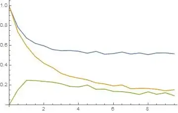
Consider the following fake data - in the actual example I'm just using more data points, but the question is still the same:
adata={{0., 0.993432}, {0.5, 0.785497}, {1., 0.675947}, {1.5, 0.622309}, {2., 0.596957}, {2.5, 0.559564}, {3., 0.548175}, {3.5, 0.549567}, {4., 0.542219}, {4.5, 0.522285}, {5., 0.541087}, {5.5, 0.512443}, {6., 0.518616}, {6.5, 0.534531}, {7., 0.513784}, {7.5, 0.524807}, {8., 0.508425}, {8.5, 0.524931}, {9., 0.525452}, {9.5, 0.516443}};
bdata={{0., 1.00119}, {0.5, 0.736208}, {1., 0.59461}, {1.5, 0.489021}, {2., 0.420658}, {2.5, 0.376625}, {3., 0.317314}, {3.5, 0.288311}, {4., 0.2703}, {4.5, 0.253141}, {5., 0.222969}, {5.5, 0.211693}, {6., 0.191978}, {6.5, 0.200777}, {7., 0.164038}, {7.5, 0.166885}, {8., 0.16606}, {8.5, 0.157586}, {9., 0.142573}, {9.5, 0.152769}};
xdata={{0., 0.00018965}, {0.5, 0.152331}, {1., 0.247705}, {1.5, 0.24586}, {2., 0.23717}, {2.5, 0.229809}, {3., 0.212898}, {3.5, 0.186414}, {4., 0.181242}, {4.5, 0.200726}, {5., 0.157727}, {5.5, 0.159359}, {6., 0.136557}, {6.5, 0.133569}, {7., 0.122987}, {7.5, 0.104608}, {8., 0.132149}, {8.5, 0.107217}, {9., 0.122394}, {9.5, 0.0933644}};

ListLinePlot[{a,b,x}]
Method 1
Use ParametricNDSolve (or ParametricNDSolveValue) to leave unevaluated those parameters that are to fit, and then use NonLinearModelFit over that InterpolatingFunction (similar to this).
transformedData={{1, 0., 0.993432}, {1, 0.5, 0.785497}, {1, 1., 0.675947}, {1, 1.5, 0.622309}, {1, 2., 0.596957}, {1, 2.5, 0.559564}, {1, 3., 0.548175}, {1, 3.5, 0.549567}, {1, 4., 0.542219}, {1, 4.5, 0.522285}, {1, 5., 0.541087}, {1, 5.5, 0.512443}, {1, 6., 0.518616}, {1, 6.5, 0.534531}, {1, 7., 0.513784}, {1, 7.5, 0.524807}, {1, 8., 0.508425}, {1, 8.5, 0.524931}, {1, 9., 0.525452}, {1, 9.5, 0.516443}, {2, 0., 1.00119}, {2, 0.5, 0.736208}, {2, 1., 0.59461}, {2, 1.5, 0.489021}, {2, 2., 0.420658}, {2, 2.5, 0.376625}, {2, 3., 0.317314}, {2, 3.5, 0.288311}, {2, 4., 0.2703}, {2, 4.5, 0.253141}, {2, 5., 0.222969}, {2, 5.5, 0.211693}, {2, 6., 0.191978}, {2, 6.5, 0.200777}, {2, 7., 0.164038}, {2, 7.5, 0.166885}, {2, 8., 0.16606}, {2, 8.5, 0.157586}, {2, 9., 0.142573}, {2, 9.5, 0.152769}, {3, 0., 0.00018965}, {3, 0.5, 0.152331}, {3, 1., 0.247705}, {3, 1.5, 0.24586}, {3, 2., 0.23717}, {3, 2.5, 0.229809}, {3, 3., 0.212898}, {3, 3.5, 0.186414}, {3, 4., 0.181242}, {3, 4.5, 0.200726}, {3, 5., 0.157727}, {3, 5.5, 0.159359}, {3, 6., 0.136557}, {3, 6.5, 0.133569}, {3, 7., 0.122987}, {3, 7.5, 0.104608}, {3, 8., 0.132149}, {3, 8.5, 0.107217}, {3, 9., 0.122394}, {3, 9.5, 0.0933644}};
sol = ParametricNDSolveValue[{
a'[t] == -k1 a[t] b[t] + k2 x[t], a[0] == 1,
b'[t] == -k1 a[t] b[t] + k2 x[t] - k3 b[t] x[t], b[0] == 1,
x'[t] == k1 a[t] b[t] - k2 x[t] - k3 b[t] x[t], x[0] == 0
}, {a, b, x}, {t, 0, 10}, {k1, k2, k3}
];
model[k1_, k2_, k3_][i_, t_] :=
Through[sol[k1, k2, k3][t], List][[i]] /;
And @@ NumericQ /@ {k1, k2, k3, i, t};
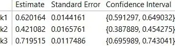
fit = NonlinearModelFit[
transformedData,
model[k1, k2, k3][i, t],
{k1, k2, k3}, {i, t}
];
Print[fit["ParameterConfidenceIntervalTable"]];
Method 2
Write the equations of the system but what is fitted are not the differential equations, but algebraic ones. This would just implying writing the right-hand part of this same example while not explicitly writing the independent variable, similarly to what is in the documentation for NonLinearModelFit.
(...updating with a working example...)
Questions
- Do you see a major difference in the possible results that these fittings could yield?
- If so, would you recommend using one over the other?
Thanks