Applying N to the roots found by Solve gives complex numbers when the roots are real

Question

I have a function which is

f(x) = x^3 - 5 x^2 - x + 1.

When I solve for x to find the zeros

Solve[x^3 - 5 x^2 - x + 1 == 0, x]
N[%]

it gives the answers

{{x -> 2.36147 - 1.11022*10^-16 I}, {x -> -2.52892 + 0. I}, {x -> 0.167449 + 0. I}}

and I want to plot these points on the graph but I don't get accurate results. please help!

Answer 1

My first observation is that

{{x -> 2.36147 - 1.11022*10^-16 I}, {x -> -2.52892 + 0. I}, {x -> 0.167449 + 0. I}}

is not a set of solutions for

 x^3 - 5 x^2 - x + 1 == 0

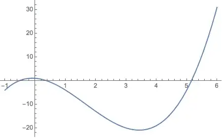
This can be seen by plotting the polynomial

Plot[x^3 - 5 x^2 - x + 1, {x, -1., 6.}]

However, the problem of imaginary fuzz in the roots remains.

Solve[x^3 - 5 x^2 - x + 1 == 0, x] // N

{
  {x -> -0.525428 - 4.44089*10^-16 I}, 
  {x -> 0.369102 + 6.66134*10^-16 I}, 
  {x -> 5.15633 - 1.4803*10^-16 I}
}

Solve takes a token, Reals, which instructs it constrain solutions to be over the real numbers. This will eliminate numeric imaginary fuzz.

Solve[x^3 - 5 x^2 - x + 1 == 0, x, Reals] // N

{{x -> -0.525428}, {x -> 0.369102}, {x -> 5.15633}}

Why is there a difference? In the first case, Solve returns a complex expression involving cube roots. Then, when N is applied, the machine numerics used for taking the cube root expressions produce a small error in the imaginary part. In the second Solve avoids the cube roots and returns Root objects.

The imaginary free result can also be achieved with

 Solve[x^3 - 5 x^2 - x + 1 == 0, x, Cubics -> False] // N