3

Here's the problem:

For one of my classes, we're supposed to use Mathematica to solve the equation y''=y-b*y' for a variety of b values and specified boundary conditions and plot the outputs. There I have no problem and Mathematica runs well. However, the next problem is to replace the -b*y' with -b*sign(y') and repeat part one. When I do this, Mathematica runs for a long time, then gives up and outputs the input. I tried removing the boundary conditions and just doing the general solution, but it can't figure that out, either. It isn't giving any errors, it just doesn't work. Any ideas? This is what my input looks like:

In[5]:=  beta = 0.2;
         Solution = DSolve[{y''[x] == - y[x] - beta * Sign[y'[x]], y[0] == 1, y'[0] == -1}, y[x], x]
Out[6]= DSolve[{y''[x] == -0.2 Sign[y'[x]] - y[x], y[0] == 1, y'[0] == -1}, y[x], x]
Rachel
  • 33
  • 2
  • Try NDSolve for {x, 0, 20}? – Michael E2 Sep 25 '14 at 18:52
  • Here's a question: does the homework specifically ask for an analytic solution to the boundary value problem, or does it only ask for the visual plots? If you're only interested in plotting the results, then replacing the symbolic DSolve with the numerical NDSolve will work better. DSolve is symbolic, and thus it may take a long time (or forever) to find a symbolic solution, whereas NDSolve is numerical, and thus is not (usually) subject to such complications. – DumpsterDoofus Sep 25 '14 at 19:13

5 Answers5

4

Try to solve the problem numerically

beta = 0.2;

As you have observed, the problem is not solved in symbolic form:

Solution = 
 DSolve[{y''[x] == -y[x] - beta*Sign[y'[x]], y[0] == 1, y'[0] == -1}, y[x], 
  x] 

(* -> DSolve[{(y^\[Prime]\[Prime])[x] == -0.2 Sign[Derivative[1][y][x]] - y[x], 
  y[0] == 1, Derivative[1][y][0] == -1}, y[x], x] *)

Now using NDSolve for x in the interval 0 to 10 (say):

yy[x_] = y[x] /. NDSolve[{y''[x] == -y[x] - beta*Sign[y'[x]], y[0] == 1, y'[0] == -1}, y[x], {x, 0, 10}] [[1]]

(* InterpolatingFunction[{{0.`,10.`}},"<>"][x] *)

This works well, and the plot looks good

Plot[yy[x], {x, 0, 10}]

(* 140925_plot_yy.jpg *)

enter image description here

The following part has been edited because of an error (26.09.14 00:52):

The solution lookes like a damped oscillation. We can try to derive the behaviour of the solution for large x as follows:

Multiplying the differential equation by y' and observing y' Sign(y') = Abs(y') we have

$y' y'' = - y y' - beta |y'|$

which can be written as

$\frac{1}{2} \frac{d}{dx} (y'^2 + y^2) = - beta |y'|$

Up to this point the reasoning is ok but in the following there is a flaw. Now, assuming $beta > 0$ the right hand side is always $<0$ which means that the expression $\frac{1}{2} (y'^2 + y^2)$ is only decreasing with x, which means that it will go to 0 which means in turn that $y\to 0$

Sorry, I shall clarify the asymptotic behaviour later.

Hope this helps, Regards Wolfgang

Dr. Wolfgang Hintze
  • 13,039
  • 17
  • 47
4

Edit 2: I think I've figured out how NDSolve constructs the solution, which has been incorporated in the revision below.

Introduction

The term -beta Sign[y'[x]] is discontinuous when beta != 0, so the IVP is not guaranteed to have a solution. NDSolve does not indicate that, but it is obvious. In such cases NDSolve automatically processes the discontinuity (references given below). This confused me for a while, but now I think I've figured it out.

Second, the differential equation alternates between $$(y - \beta)'' = -(y - \beta) \quad\hbox{and}\quad (y + \beta)'' = -(y + \beta)$$ depending on the sign of $y'$. The solution to each is a sine curve with an axis of symmetry $y = \pm \beta$, respectively. When the differential equation has a solution, it will consist of a continuous sequence of half periods of sine curves. Each half period will cover an interval (of length $\pi$) where $y'$ does not change sign; therefore the curve itself will stretch between two consecutive extrema. Over consecutive segments, $y'$ changes sign and the axis of symmetry shifts by $2\beta$. This has the effect of subtracting $2\beta$ from the amplitude. This can continue until the amplitude is less than $2\beta$, which can happen for only finitely many steps. When the amplitude would be less than $2\beta$, there is no solution, that is to say, a solution can exist only over interval of the form $(-\infty, x_0)$. Edit 1: I should add that there is a special case in which a solution can be extended to the whole real line. When the amplitude of the sine curve is an odd multiple of $\beta$, the amplitude will step down until it equals $\beta$; at the end of the interval the solution will satisfy y(x_0) = y'(x_0) = 0 and the solution can be extended to $y(x) = 0$ for all $x > x_0$. (For an example, change the initial conditions below to ics = {y[0] == 6/5, y'[0] == 0} for beta = 0.2. The initial amplitude will be 5 beta because the axis of symmetry will be y == beta.)

On the other hand, NDSolve, which I suggested in a comment, creates a solution that becomes a nonzero constant after the amplitude falls below 2 beta. That seemed curious, especially since there is no message indicating that the solution might be wrong.

ode[beta_] := y''[x] == -y[x] - SetPrecision[beta, 100]*Sign[y'[x]];
ics = {y[0] == 1, y'[0] == -1};
residual[beta_] := ode[beta] /. Equal -> Subtract;

Manipulate[
 Solution = NDSolve[{ode[beta], ics}, y, {x, 0, 20}, WorkingPrecision -> 20];
 Plot[{y[x], y'[x], -beta Sign[y'[x]]} /. First[Solution] // Evaluate,
  {x, 0, 20}, PlotRange -> All, 
  GridLines -> {ArcTan[-1 + beta, 1] + Pi Range[0, 6], beta Range[-5, 5]}, 
  PlotLegends -> {y[x], y'[x], -beta Sign[y'[x]]},
  Prolog -> {ColorData[97, 3], Dashed, 
    Line[Thread /@ {{#, y[First@#]}, {#, y[Last@#]}}] & /@ 
      Partition[ArcTan[-1 + beta, 1] + Pi Range[0, 5], 2, 1] /. First@Solution}],
 {{beta, 0.2}, 0, 2},
 TrackedSymbols :> Manipulate
 ]

Mathematica graphics

With WorkingPrecision -> MachinePrecision instead of arbitrary precision, there is some jumping around of the sign of y'[x], which is what I would expect if numerical integration is continued beyond the end point of the domain of the true solution. (When the sign of y'[x] changes and Abs[beta] > Abs[y[x]], then sign of y''[x] changes, and drives y'[x] back toward zero.)

Mathematica graphics

The residual from the ode tracks well up until ArcTan[-1 + 0.2, 1] + 3 Pi or 11.6703, at which point it is about 0.12, the same as the value of y[x] for x > 11.6703.

Block[{beta = 0.2},
 LogPlot[residual[beta] /. First@Solution // Abs,
   {x, 0, 20}, GridLines -> {ArcTan[-1 + beta, 1] + Pi Range[0, 6], None}]
 ]

Mathematica graphics

At any point there are three possibilities for Sign[y'[x]], namely -1, 0, 1. If the solution reaches a point where y'[x] == 0 and Abs[y[x]] < beta, then y'[x] could decrease, remain the same, or increase. Given that y''[x] has a value, there is only one choice, but it won't satisfy the ode. But the other possibilities won't satisfy the ode either, as shown by the residual for each choice not equaling zero:

residual[beta] /. Sign[y'[x]] -> {-1, 0, 1} /. First@Solution /. x -> 12.
(* {-0.319375, -0.119375, 0.0806248} *)

Why does NDSolve fail to give a warning?

Answer: NDSolve uses Filippov continuation automatically when discontinuous functions such as Sign appear explicitly in the differential equation. See the tutorial Events and Discontinuities in Differential Equations. This automatic processing of discontinuous functions can be turned off with the option Method -> {"DiscontinuityProcessing" -> False}.

NDSolve[{ode[0.2], ics}, y, {x, 0, 20}, 
  Method -> {"DiscontinuityProcessing" -> False}, 
  "ExtrapolationHandler" -> {Indeterminate &}];

NDSolve::mxst: Maximum number of 887537 steps reached at the point x == 11.677314840499118`. >>

In this case the phase vector field points in exactly opposite directions along y' == 0 for -beta < y < beta, so that the solution (and its continuation) is stationary:

Block[{beta = 0.2},
 StreamPlot[{p, -y - beta*Sign[p]}, {y, -2 beta, 2 beta}, {p, -2 beta, 2 beta},
  Axes -> True, Epilog -> {Red, PointSize[Large], Point[{{beta, 0}, {-beta, 0}}]}]
 ]

Mathematica graphics

From the first answer -- The following detects the problem faster. I suspect this is because the discontinuity occurs where y'[x] is zero, and therefore high Accuracy accuracy would be difficult to achieve with MachinePrecision.

One can get NDSolve to integrate up to ArcTan[-1 + 0.2, 1] + 3 Pi and give one of two warnings if AccuracyGoal is set to Infinity or to a high enough value:

NDSolve[{ode[0.2], ics}, y, {x, 0, 20}, AccuracyGoal -> Infinity]

NDSolve::ndtola: A component of the solution at x == 11.670315306734453` is essentially zero and the tolerance specified by the AccuracyGoal option could not be achieved. >>

NDSolve[{ode[0.2], ics}, y, {x, 0, 20}, AccuracyGoal -> 40]

NDSolve::ndsz: At x == 11.670315306734453`, step size is effectively zero; singularity or stiff system suspected. >>

Conclusion

It's a very interesting homework problem. If it's for an introductory undergraduate course in differential equations, I suspect a complete solution would not be expected. One of the problems with using computers to solve problems is that there is a tendency to take the answer and run with it. One sometimes forgets to think about the problem and the answer and to think of a way to check them. Perhaps that will be the "moral of story," so to speak, when your instructor reviews the assignment.

Michael E2
  • 235,386
  • 17
  • 334
  • 747
  • (at) Michael E2: I have outlined before in my solution how to proceed in general. I was stuck because I couldn't assess the asymptotic behaviour. I thought to have proved that y->0 for x->oo. But the numeric results looked different, as you have also confirmed afterwards. To be continued ... – Dr. Wolfgang Hintze Sep 26 '14 at 18:29
  • @Dr.WolfgangHintze Yes I suppose we both worked on it away from the site. I thought the conclusion that $y \rightarrow \infty$ was perhaps wrong, so I was waiting for you to finish your second answer before reading it. There are still issues to address, but I'm doubtful that it is worth the time (well, my time, at least). For instance, the solution above does not have a second derivative when the sign of y'[x] changes. If the solution is not twice-differentiable, it is not clear we can call it a solution. – Michael E2 Sep 26 '14 at 18:45
  • (at) Michael E2: I had some trouble understanding the contant asymptotic != 0 exhibited by the numeric solutions. First I got rid of the "explosion" you have observed by smoothing out the jump. Then I had the idea of the phase space consideration which led me to the calculation of the exact asymptotic value of y. My own argument of the never increasing distance of the system point from the origin in phase space turned out to be decisive in an unexpected way. Please read my answer #3 for details. – Dr. Wolfgang Hintze Sep 26 '14 at 22:19
2

Wolfgang's answer #3

It seems apropriate to create a new answer because the idea of my second answer is not taken up here.

Abstract

We present here the complete analytic solution of the problem. First we consider the problem with the sharp step replaced by a smooth one. Then a study of the phase space trajectories of the system will give the key insight into the solution. Here we conclude that the system stops after a finite sumber of oscillations. This also solves the tricky problem of the asymptotic behaviour of y. Finally, the "time" dependence is calculated which completes the solution. All this is done for the case b=0.2 but the method is general.

Smoothing out the step

Let us take instead of Sign the smooth function ArcTan so that the diffenrential equation becomes

eq = y''[x] + y[x] == -b 2/\[Pi] ArcTan[p y'[x]]

(* y[x] + (y^\[Prime]\[Prime])[x] == -((2 b ArcTan[p Derivative[1][y][x]])/\[Pi]) *)

Here the parameter p controls the steepness of the jump.

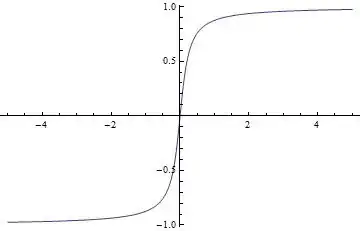
With[{p = 5}, Plot[2/\[Pi]  ArcTan[p t], {t, -5, 5}]]
(* 140926_Smooth _Step.jpg *)

enter image description here

Solving the equation with NDSolve gives for increasing steepness

yy[x_] = With[{b = 0.2, p = 5}, 
   y[x] /. First[
     NDSolve[y''[x] + y[x] == -b 2/\[Pi] ArcTan[p y'[x]] && y[0] == 1 && 
       y'[0] == -1, y[x], {x, 0, 25}]]];

Plot[yy[x], {x, 0, 25}, PlotRange -> {-1.3, 1}, 
 PlotLabel -> 
  "y(x) calculated with NDSolve for smoothed-out step\nParameters: b = 0.2, p \
= 5", AxesLabel -> {"x", "y(x)"}]

(* 140926_y(x)_smooth _p _ 5.jpg *)

enter image description here

This lookes like a normal damped oscillation.

But now p = 50 leads to a different behaviour:

yy[x_] = With[{b = 0.2, p = 50}, 
   y[x] /. First[
     NDSolve[y''[x] + y[x] == -b 2/\[Pi] ArcTan[p y'[x]] && y[0] == 1 && 
       y'[0] == -1, y[x], {x, 0, 25}]]];

Plot[yy[x], {x, 0, 25}, PlotRange -> {-1.3, 1}, 
 PlotLabel -> 
  "y(x) calculated with NDSolve for smoothed-out step\nParameters: b = 0.2, p \
= 50", AxesLabel -> {"x", "y(x)"}]
(* 140926_y(x)_smooth _p _ 50.jpg *)

enter image description here

Now there are only three passes through zero. Afterwards y stays negative and is slowly approaching y = 0.

Letting now p=5*10^3

yy[x_] = With[{b = 0.2, p = 5*10^3}, 
   y[x] /. First[
     NDSolve[y''[x] + y[x] == -b 2/\[Pi] ArcTan[p y'[x]] && y[0] == 1 && 
       y'[0] == -1, y[x], {x, 0, 25}]]];

Plot[yy[x], {x, 0, 25}, PlotRange -> {-1.3, 1}, 
 PlotLabel -> 
  "y(x) calculated with NDSolve for smoothed-out step\nParameters: b = 0.2, p \
= 5,000", AxesLabel -> {"x", "y(x)"}]
(* 140926_y(x)_smooth _p _ 5k.jpg *)

enter image description here

Leads to a constant asymptotic values <0 for y.

yy[20]

(* -0.115909 *)

Comparing this with the sharp step

yy[x_] = With[{b = 0.2}, 
   y[x] /. First[
     NDSolve[y''[x] + y[x] == -b Sign[y'[x]] && y[0] == 1 && y'[0] == -1, 
      y[x], {x, 0, 25}]]];

Plot[yy[x], {x, 0, 25}, PlotRange -> {-1.3, 1}, 
 PlotLabel -> 
  "y(x) calculated with NDSolve for sharp step\nParameter: b = 0.2", 
 AxesLabel -> {"x", "y(x)"}]
(* 140926_y(x)_sharp.jpg *)

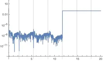
During evaluation of In[438]:= NDSolve::mxst: Maximum number of 10000 steps reached at the point x == 11.670368725029757`. >>

enter image description here

shows a breakdown of NDSolve as mentioned by Michael E2 but this happens at the same constant value of y which in the smoothed-out case is extended by NDSolve to large values of x.

Now this numeric result for the asymptotic behaviour needs to be verified independently because I have shown analytically earlier for the original Sign-function that

1/2 d/dx( y'^2 + y^2 ) = - b | y' |

Which means that the quantity y'^2 + y^2 cannot grow with increasing x. At first I thought it should go to zero together with |y'|, but this is not conclusive.

Can the equation of motion have a constant solution ya? The answer is yes: we have then y'' -> 0. This would ya -> - b Sign[y']. Now assume that for some x > x0, y' has a small positive value, i.e. Sign[y'] = +1 this leads to ya-> -b even if now y'->+0.

Now there is no contradiction: the left hand side 1/2 d/dx( y'^2 + y^2 ) -> 1/2 d/dx( 0 + y^2 ) = 1/2 d/dx( y1^2 ) = 0 and the right hand side -b |y'| -> 0 as well.

We shall make this more exact in the next section.

Phase space and asymptotics

Instead of pursuing my proposal with the piecewise trig functions (as in my soluton #2) let us look at the phase space (y, y'=v) of the problem.

The equation of motion is replaced by the system

dy/dx = v dv/dx = - y - b Sign(v)

The trajectories in phase space are given by dividing these two equations which leads to

dv/dy = - (y + b Sign(v))/v

For v<0 we have

dv/dy = - (y - b)/v

this can be integrated to give

v^2 + (y-b)^2 = const

This means the trajectories in the lower v-plane are circles centered at (y,v) = (b,0). The radius r1 is determined by the initial condition at x = 0: v(0) = -1, y(0) = 1, i.e.

r1 = Sqrt(1 + (1-b)^2)

Similarly, in the upper v-plane the trajectories are circles centered at (y,v) = (-b,0).

Let's draw a picture and look at the development of our example in phase space.

With[{b = .2},
 r1 = Sqrt[1 + (1 - b)^2]; w = ArcCos[(1 - b)/r1];
 pE = {r1 - 7 b, 0};
 pD = {-r1 + 5 b, 0};
 pC = {r1 - 3 b, 0};
 pB = {-r1 + b, 0};
 pA = {1, -1}; 
 Show[Graphics[{Line[{{-1.2, 0}, {1.2, 0}}], 
    Line[{{0, -1.5}, {0, 1}}], 
    Point[{0, 0}], {PointSize[Medium], Point[{b, 0}], 
     Point[{-b, 0}]}, {PointSize[Medium], RGBColor[1, 0, 0], 
     Point[pA], Point[pB], Point[pC], Point[pD], Point[pE]}, 
    Circle[{b, 0}, r1, {\[Pi], 2 \[Pi] - w}], 
    Flatten[Table[
      Circle[{-b, 0}, Abs[r1 - (4 k - 2) b], {0, \[Pi]}], {k, 1, 2}], 
     1], Flatten[
     Table[Circle[{b, 0}, Abs[r1 - 4 k b], {\[Pi], 2 \[Pi]}], {k, 1, 
       1}], 1], {Dashed, 
     Circle[{b, 0}, Abs[r1 - 8 b], {\[Pi], 2 \[Pi]}]}, 
    Text["A = {1,-1}", {1, -0.9}], Text["B", {-r1 + b - 0.1, 0.1}], 
    Text["C", {r1 - 3 b + 0.1, 0.1}], 
    Text["D", {-r1 + 5 b - 0.05, 0.1}], 
    Text["E", {r1 - 7 b + 0.05, 0.1}], Text["-b", {-b, 0.2}], 
    Text["b", {b, 0.2}], Text["v", {0, 1.1}], Text["y", {1.4, 0}]}]]]
(* 140926_Graph _phase-space.jpg *)

enter image description here

The system point P = (y,v) moves along successive circles of given center and radius as shown in the following table

$\left( \begin{array}{cccc} \text{segment} & \text{center} & \text{radius} & \text{y of end point} \\ A\to B & \{b,0\} & \text{r1=Sqrt[1+(1-b)${}^{\wedge}$2]} & \text{-r1+b} \\ B\to C & \{-b,0\} & \text{r2=r1-2b} & \text{r1-3b} \\ C\to D & \{b,0\} & \text{r3=r1-4b} & \text{-r1+5b} \\ D\to E & \{-b,0\} & \text{r4=r1-6b} & \text{r1-7b} \\ \end{array} \right)$

The journey stops at E = {r1-7b,0}. Why? Well, as we have shown, the distance of our system point P from the origin must never increase for increasing x. This condition is indeed met along the whole path from A to E, but would be violated if P would enter the dashed circle.

Hence the asymptotic value ya of y is reached after a finite time and is given by ya = r1 - 7b = Sqrt[1+(1-b)^2] - 7b /.b->0.2 = -0.119375. This value is now very close to the one observed with NDSolve.

I think this detailed study of the example showed all the ingredients necessary to find the asymptotic value of the solution. It would require just more labour to explore the behaviour for other values of b, especially the number of transits and hence the sign of the asymptotic value.

Also the "time" dependence of y, i.e. y(x), can be obtained easily from the phase space trajectory integrating the equation dy/dx = v giving x(y) = Integrate[1/v[y],y]. But this integral with an integrand of the type 1/Sqrt[ r^2 - (y \[PlusMinus] b)^2] is elementary and gives an ArcSin which leads to the time dependent solution which consists of segments:

y[k](x) = \[PlusMinus] b + r[k] Sin[x + c[k]]    
v[k](x) = r[k] Cos[x + c[k]]

for

x[k-1] <= x < x[k]

k = 1, 2, ..., kmax

Here r[k] are given in the table,

x[0] = 0, x[k] = Pi(k-1/2)+ArcSin[(1-b)/r[1]],

c[k] are constants determined by yk = y-value of the end point in the table.

kmax = 4 in our case.

I leave it for the interested reader to write down the explicit expressions and compare them with the previous results.

PS: I should remark that the procedure presented here improves and even replaces my solution attempt #2.

A surprisingly fascinating problem !

Regards, Wolfgang

Dr. Wolfgang Hintze
  • 13,039
  • 17
  • 47
  • I like the way your phase diagram explains why the amplitude steps down by $2\beta$ over an interval of length $\pi$. It's easier to see than my explanation. 2. Somehow I'm not seeing how the smoothed equation illuminates the OP's problem. The solution for p = 5000 approaches zero, not a negative constant. (The eigenvalues of the linearization are $(-p \pm \sqrt{p^2-25\pi^2})/(5\pi)$, whose real components are negative.) 3. By "equation of motion", do you mean the OP's DE, or the one multiplied by $y'$? Note that if a DE is multiplied by $y'$, any constant trivially becomes a solution.
  • – Michael E2 Sep 27 '14 at 19:20
  • ad 1. thanks. But the main result is that for the asymptotic value ya of y which is given by ya = Sqrt[1+(1-b)^2] - 7b /.b->0.2 = -0.119375. ad 2. first of all it seems a valid extension of the problem to be considered. Then, from the sequence of my graphs you can see that the asymptotic value is different from zero over an increasingly longer time as the steepness increases. This observation convinced me that ya !=0 which I then showed and calculated by means of the Phase space diagrams. ctd. in next comment. ad 3. I mean the original equation y''+ y = - b Sign[y']. – Dr. Wolfgang Hintze Sep 29 '14 at 06:42
  • ad 2. ctd: On the other hand, you are right, that for every finite p the asymptotic value is zero as can easily be seen from the approximation ArcTan[z] ~= z. Then y''+y = - 2/Pi b p y', and y = Exp[I w x] leads to w1 = I pb/Pi (1+Sqrt[pi^2/(pb)^2 -1], w2 = I pb/Pi (1-Sqrt[pi^2/(pb)^2 -1], and for p->oo: w1 ~= I 2pb/pi, w2 ~= I pi/(2pb). This means that from w2 y has an additive term Exp[-x pi/(2bp)] which decays exponentially the slower the larger p becomes. – Dr. Wolfgang Hintze Sep 29 '14 at 06:59
  • ad 2, ctd 2: Let me add that there is no difficulty with the approximation ArcTan(y' p) ~= y'p and p>>1. In fact, the approximation is valid for |y'p|<<1. But for the slowly decaying part, y~Exp[-x pi/(2bp)], we have |y'p| = |y p pi/(2bp)| = |y pi/(2b)| << 1 i.e. |y|<<(2/pi) b while p cancels out. – Dr. Wolfgang Hintze Sep 29 '14 at 16:47
  • I take it, however, that p >> 1 no longer "leads to a constant asymptotic values <0 for y," since we seem to agree that y -> 0, right? And if the equation of motion is the OP's $y''+y=-\beta ,\hbox{Sign}[y']$, then there are no nontrivial constant solutions, since a constant $y$ does not satisfy the differential equation ($\hbox{Sign}[y']=0$ for $y'=0$ in Mathematica). Do we agree about that? Now the smoothed DE is the explanation for Filippov's continuation method mentioned in the NDSolve documentation. Is that what you're talking about? – Michael E2 Sep 29 '14 at 17:07
  • I tend to agree with ya=0 but I still don't see how to reconcile this with the phase space picture (with the motion doublessly (?) being restricted to arc of circles around +-b). Do you consider my phase space development correct? If so, could you tell how to continue beyond point E in phase space without violating the condition that (y'^2+y^2) must not increase in time? How can the point "crawl" to (0,0)? – Dr. Wolfgang Hintze Sep 29 '14 at 18:27
  • I agree with the phase space development up to the point E and with the condition that $(y')^2+y^2)$ is nonincreasing. My conclusion is that the solution stops dead at E. There is no theorem (that I know) guaranteeing a solution in a neighborhood of E because of the discontinuity of Sign[v]. One can apply Filippov's method of continuation like NDSolve, but the continuation does not satisfy the DE. In some cases, it can be reasonable or even model reality. The continuation here is $y(x)=-0.119375$, $y'(x)=v=0$ for all future $x$, i.e. it stays at E. The position does not approach $(0,0)$.... – Michael E2 Sep 29 '14 at 18:47
  • ...You might look at the StreamPlot in my answer, which is a version of your phase plot. Over $-\beta < y < \beta$, the phase vector field is qualitatively quite different near $v = 0$ than for $y < -\beta$ or $y > \beta$. Another remark: If we look at the phase space of the smoothed DE as varying continuously with the parameter $p$, then the limit as $p\rightarrow\infty$ shows a discontinuous break. For instance, the equilibrium position $(y,v)=(0,0)$ of the smooth systems catastrophically splits into two equilibria $(y,v)=(\pm\beta,0)$ in the OP's DE. – Michael E2 Sep 29 '14 at 18:53
  • You second last comment resproduces exactly my conclusions (I quote: Hence the asymptotic value ya of y is reached after a finite time and is given by ya = r1 - 7b = Sqrt[1+(1-b)^2] - 7b /.b->0.2 = -0.119375. This value is now very close to the one observed with NDSolve.) So I agree. 2) However I still wonder why ya is not a solution of the DE, but +-b. 3) Referring to another point of the discussion: The solution y==0 of the DE is "of measure 0" as is the point 0 in Sign and is not reached in the time development. ctd.
  • – Dr. Wolfgang Hintze Sep 30 '14 at 06:03
  • Your discussion of the catastrophic splitting of the equilibirum point (0,0) is interesting; and it shows the value of the smoothed DE. But as I asked in the first part of this comment: why +-b rather than Sqrt[1+(1-b)^2] - 7b ?
  • – Dr. Wolfgang Hintze Sep 30 '14 at 06:09