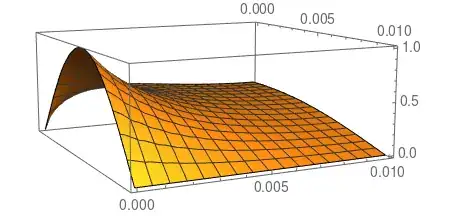
I would like to solve the following nonlinear coupled PDE with a mix of initial conditions and boundary values:
rMax = 0.01;
sol = First@NDSolve[{
Derivative[2, 0][g][r, z] + Derivative[0, 2][g][r, z] == u[r, z]^2,
Derivative[2, 0][u][r, z] + Derivative[0, 1][u][r, z] == -g[r, z],
Derivative[1, 0][u][0, z] == 0.0,
Derivative[1, 0][u][rMax, z] == 0.0,
u[rMax, z] == 0.0,
u[r, 0] == g[r, 0] == Sin[\[Pi] r/rMax],
Derivative[1, 0][g][0, z] == g[rMax, z] == 0.0},
{u, g}, {r, 0, rMax}, {z, 0, 0.01}]
but I receive the following error message (in version 10.0.1.0):
NDSolve::femnonlinear: Nonlinear coefficients are not supported in this version of NDSolve.
The offender is the square term u[r, z]^2 in the first equation; without the square NSolve[] executes without errors. NDSolve seems to apply the FEM method by default to such problems. I'm wondering why NDSolve[] doesn't switch back to another (propagation-type) algorithm? When I add the option Method -> "MethodOfLines", the error message changes to
NDSolve::ivone: Boundary values may only be specified for one independent variable. Initial values may only be specified at one value of the other independent variable.
and I don't quite understand why this is because my time-like variable is z and I'm setting initial conditions only for z=0 and then boundary conditions at r=0 and r=rMax which should be OK?
Any ideas how to solve my problem? Another post suggested calling low-level FEM routines directly, is this a solution? What's the advantage of using FEM on an initial condition/boundary value problem over other methods: speed, accuracy, robustness?

NDSolve[..., Method -> {"MethodOfLines", "TemporalVariable" -> z}]-- You'll get another error message, but perhaps that will give you a clue. – Michael E2 Sep 26 '14 at 14:51NDSolve::tvic: "z cannot be used as the temporal independent variable because the conditions {u[r,0]==Sin[6283.19\ r],g[r,0]==Sin[6283.19\ r]} for that dimension do not constitute sufficient initial conditions given at only one value of z."Why would the condition at z=0 not be sufficient, being at the beginning of the requested solution range? – RonH Sep 26 '14 at 15:07z == 0? – Michael E2 Sep 26 '14 at 15:08Derivative[1, 0][u][0, z] == 0condition be inconsistent withu[r, 0] == Sin[π r/rMax]? – Silvia Sep 27 '14 at 04:03Derivative[0, 1][g][r, 0] == 0.0andMethod -> {"MethodOfLines", "TemporalVariable" -> z}as you suggested. The solution is terribly slow, though, and I feel this shouldn't be the case since there's no fast variation or stiffness/singularity in the physical system I'm trying to model. I added the optionsAccuracyGoal -> 3, PrecisionGoal -> 3, MaxSteps -> 10^5. Do you think it's worth playing with the discretization method, specify a grid size etc.? – RonH Sep 29 '14 at 11:15Cos[Pi/2 r/rMax], I still get inconsistent boundary and initial conditions (forDerivative[1, 0][u][rMax, z] == 0). – Michael E2 Sep 29 '14 at 13:09