How to measure cross-covariance in mathematica

Question

In matlab cross-covariance is given by [c,lags] = xcov(x,maxlags,'coeff'); How can I measure in Mathematica?

Answer 1

Update

a Rewrite of my answer in an effort to recreate Matlab's xcov function. I'm using this documentation page as reference. I'd appreciate any code review, in particular how the scale options are implemented since I've seen conflicting documentation. First, the function:

Clear[CrossCovariance];
Options[CrossCovariance] = {"Lag" -> All, "Scale" -> None};
CrossCovariance::lagtoolarge = 
  "The option for Lag (`1`) is greater than the length of the Lists \
provided. Using maximum possible Lag";
CrossCovariance[x_List, opts : OptionsPattern[]] := 
 If[Length@Dimensions[x] == 1, CrossCovariance[x, x, opts],
  CrossCovariance[Sequence @@ #, opts] & /@ Tuples[x, 2]]
CrossCovariance[x_List, y_List, OptionsPattern[]] := 
 Module[{nmax, xlist, ylist, scale, s},
  xlist = x;
  ylist = y;
  (* Pad the shorter list with zeros *)
  If[Length@xlist > Length@ylist, 
   ylist = PadRight[ylist, Length@xlist]];
  If[Length@xlist < Length@ylist, 
   xlist = PadRight[xlist, Length@ylist]];
(* Implement Lag option, Fixes non-integer and negative lag values *)
nmax = If[OptionValue["Lag"] =!= All, 
    IntegerPart@Abs@OptionValue["Lag"], Length@xlist - 1];
  If[nmax > Length@xlist - 1, (nmax = Length@xlist - 1; 
    Message[CrossCovariance::lagtoolarge, OptionValue["Lag"]])];
(* Implement the Scale option, None does nothing, 
  "biased" is a biased estimate, 
  "unbiased" is an unbiased estimate and "coeff" normalizes the list so that 

  autocovariance with zero lag is equal to 1. All else is assumed to be None *)
  scale = 1;
  s[n_] := Switch[
    OptionValue["Scale"],
    "unbiased", Length@xlist,
    "biased", (Length@xlist - Abs[n]),
    "coeff", 1/Covariance[xlist, ylist],
    _, 1];
(* Create CrossCovariance table *)
  Table[s[n] Covariance[xlist, RotateRight[ylist, n]], {n, -nmax, nmax, 1}]]

Now some data. s1 is random, s2 is s1 shifted by 50 places and s3 is a few short of s2; data is real periodic sunspot data from here

SeedRandom[1234];
s1 = RandomReal[1, 150];
s2 = RotateRight[s1, 50];
s3 = Drop[s2, 25];
data = Flatten@
   Import["http://w3eos.whoi.edu/12.747/notes/lect06/SUNSPOTS.DAT"];

The random data and its shifted counterpart

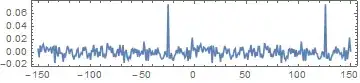
Compute the noramlized autocovariance of the the randomized data

ListLinePlot[CrossCovariance[s1, "Scale" -> "coeff"], 
 PlotRange -> All, DataRange -> {-150, 150}, Frame -> True, 
 Axes -> False, AspectRatio -> 1/5]

Lists of unequal length are dealt with using zero padding

ListLinePlot[CrossCovariance[s1, s3], PlotRange -> All, 
 DataRange -> {-150, 150}, Frame -> True, Axes -> False, 
 AspectRatio -> 1/5]

Compute the biased estimates of the autocovariance and mutual cross-covariance sequences.

ListLinePlot[CrossCovariance[{s1, s2}, "Scale" -> "biased"], 
 PlotRange -> All, DataRange -> {-150, 150}, Frame -> True, 
 Axes -> False, AspectRatio -> 1/5]

Limit the range of shifted values with "Lag". End user needs to address the symmetry around the zero-shift if desired.

cvdata = CrossCovariance[data, "Lag" -> 588, "Scale" -> "coeff"];
ListLinePlot[cvdata[[1178/2 ;;]], PlotRange -> All, 
 DataRange -> {0, 588/12}, Frame -> True, Axes -> False, 
 AspectRatio -> 1/5]

Previous version

As far as I can tell, Mathematica does not have a cross-covariance function built in. However, if we take a look at what cross-covariance is from here and there on the internet, we can come up with a method which might help you out. I'll use the first reference, which contains some example sunspot data:

data = Flatten@Import[
   "http://w3eos.whoi.edu/12.747/notes/lect06/SUNSPOTS.DAT"];

The cross-covariance of this data set (or more precisely, the auto-covariance) is the Covariance of the original dataset and a time-shifted copy. We can get at the time shifted copy using the following:

 ListLinePlot[Table[Covariance[data[[n ;;]], data[[;; -n]]], {n, 1, 588, 1}], 
   DataRange -> {0, 49}]

As expected, we see the largest covariance when there is no lag, which makes sense since the data should match up with itself perfectly. We see local maxima in the time-lagged covariance with a periodicity of about 11 years, which is consistent with the 11-year sunspot cycle we have all learned about.

Finding the cross-covariance of two stochastic processes would function the same way assuming the time steps and dataset lengths are equal.

And just for fun, compare the auto-covariance of the sunspot data with normally distributed data with the same mean and standard deviation:

datar = RandomVariate[
   NormalDistribution[Mean@data, StandardDeviation@data], 
   Length@data];
ListLinePlot[
 Table[Covariance[datar[[n ;;]], datar[[;; -n]]], {n, 1, 588, 1}], 
 DataRange -> {0, 49}, PlotRange -> All]

We see that the auto-covariance very quickly drops to 0, indicating that there is no signal contained in this dataset.