How to generate a chirped signal?

Question

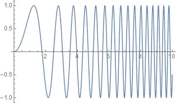
As there is no ChirpSignal function in Mathematica, can anyone tell me how to write a custom function to generate a sinusoid with a frequency that changes continuously from frequency f1 to f2 over a certain time of t?

This is what I done to generate the chirp:

{freq0, freqs, TrBandw, RCbandw, pulseLength, dt} = 
  {9 10^6, {10 10^6, 20 10^6}, 4, 10^6, 5 10^5, 2.67 10^-6, 1 10^-8};

i = 0;
nfreqs = Length@freqs;
n = Ceiling[pulseLength/dt];

fmin = freqs[[1]] - RCbandw/2;
fmax = freqs[[-1]] + RCbandw/2;

nextend = n*nfreqs;
w = 2 Pi (fmin + Range[0, nextend - 1] (fmax - fmin)/(nextend - 1));

Phi = 
  PadRight[
    Accumulate[Insert[Table[w[[i]] dt, {i, 2, n*nfreqs}], 0, 1]], 
    IntegerPart[((nfreqs + 1) pulseLength)/dt], 
    0];

s = Sin[Phi];

enter image description here

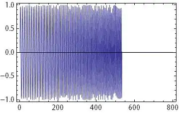
At the end, I need to filter the chirp with a Butterworth (or any other filter) to remove frequencies that do not fit in the span of [cutoff1, cutoff2]

cut1 = (freq0 - 0.5 TrBandw)/(1/dt/2)
cut2 = (freq0 + 0.5 TrBandw)/(1/dt/2)

cut1 = 0.14 Hz
cut2 = 0.22 Hz

The final result looks something like this in matlab

enter image description here

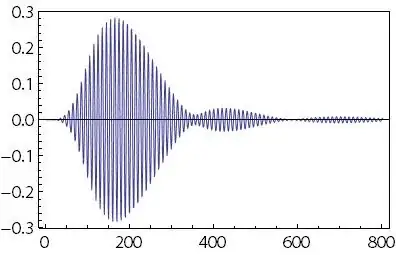
Most part of my problem lies in the filtering. So, instead of my code for the chirp, I can use the simpler approach suggested. Still, it would be great to have help with the filtering part, too.

This seems rather well addressed here: http://en.wikipedia.org/wiki/Chirp -- have you tried to implement this yourself? Where did you run into trouble? — Mr.Wizard, Oct 20 '14 at 19:38
Yes, I tried to filter the chirp with BandpassFilter command, however the amplitude of the output signal doesn't exceed +/- 0.04. — kvnF2, Oct 21 '14 at 11:05

score 14 · Answer 1 · answered Oct 20 '14 at 20:03

If you're trying to just generate a chirp over all time, you can use:

Clear[Chirp, fc, f1, tau]
Chirp[t_, fc_, f1_, tau_] := Cos[2*Pi*(fc*t + (f1 - fc)/tau*t^2)]
Plot[Chirp[t, 100, 150, 0.25], {t, 0, 0.25}]

Output 1

Basically, this is: $$ \mathcal{Re}\left\{e^{i2\pi f_ct+i2\pi\beta t^2}\right\} $$ Where $\beta$ is the rate of change in frequency (in Hz/sec). To solve for $\beta$, we just rewrite it as the change in frequency ($f_c-f_1$) over the chirp time ($\tau$). This is how the above Mathematica code is derived. If you're trying to detect a chirp, such as using correlation, you could redefine the chirp function as a piecewise function, so as to make it 0 outside of the chirp time:

Clear[Chirp, fc, f1, tau]
Chirp[t_, fc_, f1_, tau_] := Piecewise[{{Cos[2*Pi*(fc*t + (f1 - fc)/tau*t^2)], 0 <= t <= tau}}, 0]
Plot[Chirp[t, 100, 150, 0.25], {t, -0.25, 0.35}]

Output 2

Personally, I usually put the chirp in terms of $\beta$, which would make the above function

Chirp[t_, fc_, beta_, tau_] := Piecewise[{{Cos[2*Pi*(fc*t + beta*t^2)], 0 <= t <= tau}}, 0]

And if I need the Quadrature component (Which would be $ \mathcal{Im}\left\{e^{i2\pi f_ct+i2\pi\beta t^2}\right\} $)

Chirp[t_, fc_, beta_, tau_] := Piecewise[{{Sin[2*Pi*(fc*t + beta*t^2)], 0 <= t <= tau}}, 0]

Welcome to Mathematica SE! Nice detailed explanation :) – ybeltukov Oct 20 '14 at 20:07 — ybeltukov, Oct 20 '14 at 20:07

score 2 · Answer 2 · answered Oct 12 '23 at 13:14

There is now a ChirpFunction in the Wolfram Function Repository. You specify the initial and final frequencies and you get back a compiled function which you can use to quickly generate the actual signal. It has several options for customizing the chirp.

score 2 · Answer 3 · answered Oct 20 '14 at 19:34

2

Here is a start until more detail is specified:

Plot[Sin[t*t], {t, 0, 10}]

enter image description here

answered Oct 20 '14 at 19:34

Mr.Wizard

271,378
34
587
1,371

score 1 · Answer 4 · answered Nov 26 '14 at 23:55

Clear[PulseTemplateChirp];
PulseTemplateChirp[freq0_, freqs_, TrBandw_, RCbandw_, pulseLength_, 
  dt_] :=
 Block[{fmin, fmax, chirpLength0, nfreqs, 
   chirpLength, \[Phi],(*chirp0,*)cut1, cut2, tf, dtf, chirp1, cut01, 
   cut02, bwf, dbwf, chirpn, z},

  fmin = freqs[[1]] - RCbandw/2;
  fmax = freqs[[-1]] + RCbandw/2;

  chirpLength0 = Round[pulseLength/dt] + 1;
  nfreqs = Length@freqs;
  chirpLength = nfreqs chirpLength0;

  \[Phi] = PadRight[
    Accumulate[
     Insert[
      Table[
       2 \[Pi] (fmin + (fmax - fmin)/chirpLength t) dt, {t, 2, 
        chirpLength}]
      , 0, 1]
     ],
    IntegerPart[((nfreqs + 1) pulseLength)/dt], 0];

  chirp0 = Sin[\[Phi]];


  cut1 = (freq0 - 0.5 TrBandw)/0.5;
  cut2 = (freq0 + 0.5 TrBandw)/0.5;

  (*This creates a Butterworth filter with a 5 dB passband at 
  cut1<f<cut2 and -50 dB stopbands at f<(0.8cut1) and f>(2cut2)*)
  tf = ButterworthFilterModel[{"Bandpass", 
     2 \[Pi] {0.8 cut1, cut1, cut2, 2 cut2}, {50., 5.}}];
  (*Convert to discrete-time IIR filter*)
  dtf = ToDiscreteTimeModel[tf, 0.5 dt, z];
  (*Filter chirp sequence*)
  chirp1 = RecurrenceFilter[dtf, chirp0];

  chirpn =
   Reap[
     Do[
      cut01 = (freqs[[i]] - 0.5 RCbandw)/0.5;
      cut02 = (freqs[[i]] + 0.5 RCbandw)/0.5;

      bwf = 
       ButterworthFilterModel[{"Bandpass", 
         2 \[Pi] {0.9 cut01, cut01, cut02, 2 cut02}, {15., 2.}}];
      dbwf = ToDiscreteTimeModel[bwf, 0.5 dt, z];

      Sow[RecurrenceFilter[dbwf, chirp1]],

      {i, nfreqs}]
     ][[2, 1]]
  ]


chirps = PulseTemplateChirp[9 10^6, {10 10^6, 12 10^6}, 4 10^6,5 10^5, 2.67 10^-6, 1 10^-8];

ListLinePlot[chirps[[1]]]

enter image description here

How to generate a chirped signal?

4 Answers4

Linked

Related