Defining an alternative derivative function?

Question

I want to calculate the derivative at a point, but I do not want to use the built-in derivative function D.

I began with this definition of the derivative

Limit Definition of Derivative ,

which resulted in: Limit[ #, h -> 0] & /@ { (f[x + h, y] - f[x, y])/ h.

But, I want to calculate the derivative at a point with the definition

Derivative at a Point .

One aim is to increase the accuracy of the calculation by using a set of set of $x$_$i$ (a numerical grid), where the spacing from one grid point to the next is $∆x$. For example, $∆x$ = 0.001, a grid of 10,000 points ($i$ = 1, . . . , 10000) would span a spatial range of 10 units in $x$.

I'm thinking one of these forms would be ideal for $x$_$i$ ...

x_i = i∆x   
x_i = (i − i_m) ∆x  
x_i = i∆x − x_m,

but I'm not sure which is best.

Ultimately, I want to take a function $f$ of two variables, for example

f[x_, n_] := - Sum [Sin[j x] /j, {j, 1, n}],

at the grid points $x$_$i$, and run through the grid, applying the derivative at a point equation (involving two neighbors for each derivative point). Then, after having the first derivative on the entire grid, calculate the second derivative on the grid, involving two first-derivative neighbors. Finally, I want to display the results on a plot.

My first thought is to use a do loop, a couple of arrays, and ListPlot, but I'm not sure exactly how to proceed, as I've just started with Mathematica.

UPDATE: I do not want to use the Derivative or D functions. – Curious14 Nov 09 '14 at 23:03 — Curious14, Nov 09 '14 at 23:03

score 4 · Answer 1 · answered Nov 09 '14 at 19:22

4

In Mathematica, to take a derivative, grinding through Do loops, producing arrays, and defining finite-difference differentials are all completely unnecessary; instead, just use D:

Plot[Evaluate@Table[D[f[x, n], {x, 2}], {n, 1, 5}], {x, 0, 2 Pi}, PlotLegends -> "Expressions"]

which produces the graph that you are trying to make:

enter image description here

answered Nov 09 '14 at 19:22

DumpsterDoofus

11,857
1
29
49

UPDATE: I do not want to use the Derivative or D functions. – Curious14 Nov 09 '14 at 23:04

score 2 · Answer 2 · answered Nov 10 '14 at 03:05

For the first question (re finite difference from a table): Differences will compute the differences.

xlist = Range[0., 20., 0.001];
flist = Sin@xlist;

ListLinePlot[{Transpose@{xlist, flist}, 
  Transpose@{Most@xlist, Differences[flist]/0.001},
  Transpose@{Rest@Most@xlist, Differences[flist, 2]/0.001^2}}]

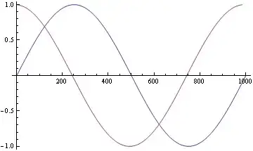
Mathematica graphics

If x is a nonuniform grid, e.g., xlist = Sort@RandomReal[{0, 100}, 10000], then you can use Differences[flist]/Differences[xlist] for the first derivative.

As for the ultimate question, I don't know what to add to DumpsterDoofus's answer. 42? The question doesn't seem to have much to do with functions defined by a numerical table/grid.

score 1 · Answer 3 · edited Apr 13 '17 at 12:55

Here you have how to perform higher order approximations, following what I did here

halfKernel = {-(8/9), 14/45, -(56/495), 7/198, -(56/6435), 2/1287, -(8/45045), 1/102960} // N;
kernel = Join[-Reverse@halfKernel, {0}, halfKernel];
t[n_] := t[n] = Table[Sin@y // N, {y, 0, 2 Pi, 2 Pi/n}]
tprime[n_] := ListConvolve[kernel, n /(2 Pi) t[n]];


ListLinePlot[{t[1000], tprime[1000]}]

Mathematica graphics

In the link above you can also find the coefficients for the second derivative

Defining an alternative derivative function?

3 Answers3