I start with the following:
sol = DSolve[{y'[t] == y[t]^2 - y[t], y[0] == c}, y[t], t];
y[t_, c_] := y[t] /. First[sol];
The output is:
Solve::ifun: Inverse functions are being used by Solve, so some solutions may not be found; use Reduce for complete solution information. >>
My first question is how do I use Reduce to obtain complete solution information? That is, what specific command should I enter?
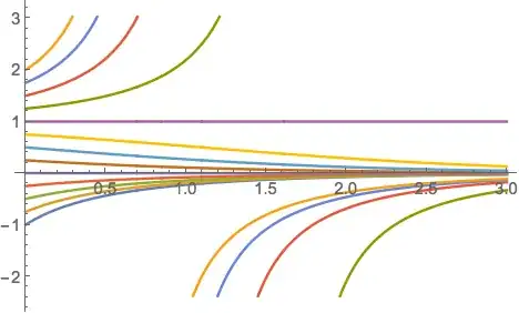
Next, I found a family of solutions.
family = Table[y[t, c], {c, -1, 2, 0.25}]
Output:
{1./(1. -2. E^t), 0.75/(0.75 -1.75 E^t), 0.5/(0.5 -1.5 E^t),0.25/(0.25 -1.25 E^t),0.,-(0.25/(-0.75 E^t-0.25)),-(0.5/(-0.5 E^t-0.5)),-(0.75/(-0.25 E^t-0.75)),1.,-(1.25/(0.25 E^t-1.25)),-(1.5/(0.5 E^t-1.5)),-(1.75/(0.75 E^t-1.75)),-(2./(1. E^t-2.))}
Then I plotted the family of solutions.
Plot[family, {t, 0, 3}, Frame -> True, FrameLabel -> {x, y}, PlotRange -> {-7, 8}]
The resulting image:

Next, I want to eliminate the vertical lines, so I tried:
dens = Denominator[family]
Output:
{1. - 2. E^t, 0.75 - 1.75 E^t, 0.5 - 1.5 E^t, 0.25 - 1.25 E^t, 1, -0.25 - 0.75 E^t, -0.5 - 0.5 E^t, -0.75 - 0.25 E^t, 1, -1.25 + 0.25 E^t, -1.5 + 0.5 E^t, -1.75 + 0.75 E^t, -2. + 1. E^t}
Then I wanted to find where each of these denominators equal zero. I got lucky with:
Map[(Solve[# == 0, t] &), dens]
Output:
Solve::ifun: Inverse functions are being used by Solve, so some solutions may not be found; use Reduce for complete solution information. >>
Solve::ifun: Inverse functions are being used by Solve, so some solutions may not be found; use Reduce for complete solution information. >>
Solve::ifun: Inverse functions are being used by Solve, so some solutions may not be found; use Reduce for complete solution information. >>
General::stop: Further output of Solve::ifun will be suppressed during this calculation. >>
But I got this output:
{{{t -> -0.693147}}, {{t -> -0.847298}}, {{t -> -1.09861}}, {{t -> \ -1.60944}}, {}, {{t -> -1.09861 + 3.14159 I}}, {{t -> 0. + 3.14159 I}}, {{t -> 1.09861 + 3.14159 I}}, {}, {{t -> 1.60944}}, {{t -> 1.09861}}, {{t -> 0.847298}}, {{t -> 0.693147}}}
I then copied and pasted the last four values with Exclusion:
Plot[family, {t, 0, 3},
 Exclusions -> {1.6094379124341003, 1.0986122886681098,
   0.8472978603872036, 0.6931471805599453}]
Which gave me the image I wanted.
What I am wondering is there a way that I could just select the real numbers that make the denominators equal to zero and slip them into the Exclusion option.
Of course, I'd also be interested in an alternate way of removing the vertical lines.
Simple Method: I got a response to a support request from Wolfram, and received a nice way that I think my students can understand.
Clear[Derivative];
Clear[y];
eqn = {y'[x] == 1 - y[x]^2, y[0] == k}

{Derivative[1][y][x] == 1 - y[x]^2, y[0] == k}
Then:
sol = DSolve[eqn, y, x]

Solve::ifun: Inverse functions are being used by Solve, so some solutions may not be found; use Reduce for complete solution information. >>

{{y -> Function[{x}, (-1 + E^(2 x) + k + E^(2 x) k)/(
    1 + E^(2 x) - k + E^(2 x) k)]}}
Then the plot:
Plot[Evaluate[Table[y[x] /. sol, {k, -2, 2, .2}]], {x, -5, 5}]

Now, noting the denominator of the solution is $1+e^{2x}-k+e^{2x}k$:
Show[Table[
  Plot[y[x] /. sol, {x, -5, 5},
   Exclusions -> 1 + E^(2 x) - k + E^(2 x) k == 0,
   PlotStyle -> Hue[k/4 + 0.5]], {k, -2, 2, .2}]]
Which provides the desired image.

Another Simple Method: Using the Denominator command and the new DSolveValue command in Mathematica 10, things are even easier:
eqn = {y'[x] == 1 - y[x]^2, y[0] == k};
sol = DSolveValue[eqn, y[x], x] // Quiet;
Show[Table[Plot[sol, {x, -5, 5},
   Exclusions -> Denominator[sol]], {k, -2, 2, .2}]]
Which gives the following image.
