13

I'm trying to use Mathematica to solve the water hammer effect.

g = 9.81;
a = 1350;
L = 3500;
h0 = 4;
v0 = Sqrt[2 g h0];
R = 0.003;

sol = NDSolve[{ D[h[x, t], x] - Rv[x, t]Abs[v[x, t]] == 1/g D[v[x, t], t], D[v[x, t], x] == g/a^2*D[h[x, t], t],

   v[x, 0] == v0,
   v[0, t] == v0 Exp[-t^2/0.4],
   h[L, t] == h0,
   h[x, 0] == h0},

  {h, v},
  {x, 0, L}, {t, 0, 10}
 ];

Manipulate[ Plot[Evaluate[v[x, t] /. sol], {x, 0, L}, PlotRange -> {-2 v0, 2 v0}], {t, 0, 10}]

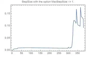
What I get near the end of the time interval is something I'm not expecting: enter image description here

The documentation tells me to use the option:

Method -> {"MethodOfLines","SpatialDiscretization" -> {"TensorProductGrid", "MinPoints" -> 750}}

but it just makes it worse.

Can somebody help me out with this one?

PS: Take R=0 and you get a lossless system, and the solution should be a wave traveling and reflecting for h and v.

Ivan
  • 2,207
  • 15
  • 25

2 Answers2

12

You need the magic of "Pseudospectral" or a dense enough 2nd order spatial difference grid:

mol[n_Integer, o_:"Pseudospectral"] := {"MethodOfLines", 
  "SpatialDiscretization" -> {"TensorProductGrid", "MaxPoints" -> n, 
    "MinPoints" -> n, "DifferenceOrder" -> o}}

g = 9.81;
a = 1350;
L = 3500;
T = 30;
h0 = 4;
v0 = Sqrt[2 g h0];
R = 0.003;

(* Solution 1 *)
sol = NDSolve[{D[h[x, t], x] - R v[x, t] Abs[v[x, t]] == D[v[x, t], t]/g, 
    D[v[x, t], x] == g D[h[x, t], t]/a^2, v[x, 0] == v0, v[0, t] == v0 Exp[-(t^2/0.4)], 
    h[L, t] == h0, h[x, 0] == h0}, {h, v}, {x, 0, L}, {t, 0, T}, Method -> mol[45]];

(* Solution 2 *)
sol2 = NDSolve[{D[h[x, t], x] - R v[x, t] Abs[v[x, t]] == D[v[x, t], t]/g, 
    D[v[x, t], x] == g D[h[x, t], t]/a^2, v[x, 0] == v0, v[0, t] == v0 Exp[-(t^2/0.4)], 
    h[L, t] == h0, h[x, 0] == h0}, {h, v}, {x, 0, L}, {t, 0, T}, Method -> mol[200, 2]];

(* Use sol2 inside Plot if you like *)
Manipulate[
 Plot[Evaluate[v[x, t] /. sol], {x, 0, L}, PlotRange -> {-2 v0, 2 v0}], {t, 0, T}]

enter image description here

Velocity at the end of the pipe:

(* Use sol2 inside Plot if you like *)
Plot[Evaluate[v[L, t] /. sol], {t, 0, T}, PlotRange -> {-2 v0, 2 v0}]

enter image description here

xzczd
  • 65,995
  • 9
  • 163
  • 468
  • Awesome! Thank you! This works great and fast enough. Could you elaborate on the "magic" part? – Ivan Dec 12 '14 at 19:42
  • 1
    @Ivan To be honest, I'm not able to… the only thing I know is that "Pseudospectral" seems to be quite effective on certain kind of PDEs (specifically speaking, PDEs related to fluid dynamics and quantum mechanics, according to the examples appearing in this site so far), but I never studied why. Maybe you can consider asking it in http://scicomp.stackexchange.com/ ? – xzczd Dec 15 '14 at 05:25
7

With the option MaxStepSize -> 1., it seems to work. (A little bit magic)

sol = NDSolve[{
           D[h[x, t], x] - R*v[x, t]*Abs[v[x, t]] == 1/g D[v[x, t], t],
           D[v[x, t], x] == g/a^2*D[h[x, t], t],

           v[x, 0] == v0,
           v[0, t] == v0 Exp[-t^2/0.4],
           h[L, t] == h0,
           h[x, 0] == h0},

          {h, v},
          {x, 0, L}, {t, 0, 10},
          MaxStepSize -> 1.
         ];

enter image description here

Here are the step sizes with the option MaxStepSize -> 1. :

enter image description here

Of course it is a way below 1...

... and It is finer that with the default MaxStepSize :

enter image description here

In the comments, @belisarius ask a plot of the velocity at the end of the pipe. Here it is :

enter image description here

andre314
  • 18,474
  • 1
  • 36
  • 69
  • @belisarius This is consistent with the simulation above. At the end of the line (x=L) there is a oscillation. The caracteristics of the oscillation depend of the length of the line. – andre314 Dec 10 '14 at 20:23
  • I'm not sure, though. I think the fluid should come to a stop due to the dissipation. – Dr. belisarius Dec 10 '14 at 20:49
  • @belisarius This is precisely what happens : when you move the cursor you see that the wave is vanishing. – andre314 Dec 10 '14 at 20:55
  • 1
    Ok, I can't run this in my machine (takes too much time). Perhaps you could include a plot of the velocity as a function of time at the end of the pipe. – Dr. belisarius Dec 10 '14 at 21:00
  • @belisarius I have added a plot of the velocity. – andre314 Dec 10 '14 at 21:09
  • Thank you! The results are what I was expecting. The only problem is the time it takes to evaluate. It takes about 2 minutes in my PC. What can be done to make it faster? – Ivan Dec 10 '14 at 23:13