Sampling a phase space uniformly for a given energy?

Question

The energy for a 1D harmonic oscillator can be written: $$ E = \frac{1}{2 m} p^2 + \frac{m \omega^2}{2} x^2 $$ where x is position and p is the momentum.

I would like to sample phase space $(x,p)$ uniformly (generating random numbers), in the case where: $$ \frac{1}{2 m} = \frac{m \omega^2}{2}, $$ trajectories with the same energy $E'$ in phase space lie in a circle centered at the origin with radius $\sqrt{2 m E'}$. Therefore, we can use the trick in this answer: uniform distribution on unit circle

In my particular problem, the energy is given by: $$ E = \frac{p_x^2 + p_y^2 + p_z^2}{2 m} + V(x,y,z) $$ where $V(x,y,z)$ is the potential energy of Cartesian co-ordinates. I would like to generate random numbers $(x,y,z,p_x,p_y,p_z)$ that are uniformly distributed in allowed phase space all with energy $E'$

...This sounds like a hard research problem. Even in your 1D example, if you don't have $\frac1{2m}=\frac{m\omega^2}2$ you're trying to sample uniformly from the boundary of an ellipse, and that's not easy. — , Dec 14 '14 at 17:50
Do you have a particular function in mind for V(x,y,z)? If not, can you state whether E = E' is a continuously differentiable closed surface? — bbgodfrey, Dec 14 '14 at 19:13
The potential I have in mind is $V(x,y,z) = c \sqrt{\frac{x^2+y^2}{4 a^2} + \frac{z^2}{a^2}}$ where $a$ and $c$ are constants. When I want to generate the random numbers, $a, c, m$ and $E$ will be some numerical value. — user29165, Dec 14 '14 at 19:48
@user29165, do you really mean to include the Sqrt, which causes V not to be analytical at the origin? I would have expected something like V [x, y, z] = c ((x^2 + y^2)/(4 a^2) + z^2/a^2), analogous to your 1D example. — bbgodfrey, Dec 14 '14 at 20:18
In my case, I do have the sqrt in the potential, I was just listing the 1d harmonic oscillator as an example as it would be familiar to most people. — user29165, Dec 14 '14 at 20:24

score 7 · Answer 1 · edited Apr 13 '17 at 12:55

Solving the one-dimensional problem is a first step toward solving the three-dimensional problem described in the question and comments. Without loss of generality, it can be written after renormalization as

1 == p^2 + Sqrt[x^2/4]

Noting that phase space is mirror-symmetric about both axes, we solve for the phase curve in the quadrant p > 0, x > 0.

xphase = x /. Assuming[x > 0, Solve[%, x]][[1, 1]];
Plot[xphase, {p, 0, 1}, AxesLabel -> {p, x}]

phase space

To "sample phase space uniformly", we compute the arc length of this curve and sample it uniformly.

dsdp = Sqrt[1 + (D[xphase, p])^2];
arc = Simplify[s[p] /. DSolve[{s'[p] == dsdp, s[0] == 0}, s[p], p][[1]]]

with solution

(4*p*Sqrt[1 + 16*p^2] + ArcSinh[4*p])/8

Knowing arc as a function of p, we compute the inverse function in the usual manner.

pinv[s_] := p /. FindRoot[arc - s, {p, .5}]

Finally, following 63805, we obtain

ListPlot[{pinv[#], xphase /. p -> pinv[#]} & /@ 
  RandomVariate[UniformDistribution[{0, arc /. p -> 1}], 100], AxesLabel -> {p, x}]

distribution

Presumably, the complete problem can be solved by generating a uniform distribution on the unit sphere in six dimensions and mapping it to the surface generated by the Hamiltonian described in the question and comments.

score 5 · Answer 2 · edited Apr 13 '17 at 12:55

Alternative 2D Solution

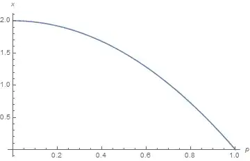
A simpler and more readily generalizable alternative to the solution presented in my previous Answer can be obtained by noting that a UniformDistribution on the curve shown in the first figure is equivalent to a ProbabilityDistribution in p weighted by dsdp,

ProbabilityDistribution[dsdp/arcmax, {p, 0, 1}]

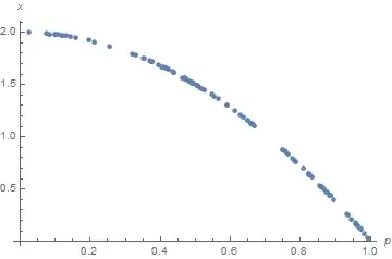
as can be can be demonstrated by

ListPlot[{#, 2 (1 - #^2)} & /@ RandomVariate[ProbabilityDistribution[dsdp/arcmax, {p, 0, 1}], 100],
  AxesLabel -> {p, x}]

which reproduces the second plot in the earlier Answer.

6D Solution (Almost)

Without loss of generality, the full problem can be written after renormalization as

1 == px^2 + py^2 + pz^2 + Sqrt[x^2/4 + y^2/4 + z^2]

Subsequent calculations can be simplified considerably by transforming momentum space to spherical coordinates and configuration space to cylindrical coordinates.

1 == p^2 + Sqrt[z^2 + r^2/4]

where p^2 = px^2 + py^2 + pz^2 and r^2 = x^2 + y^2. Noting that phase space is mirror-symmetric about all axes, we solve for the surface represented by this equation for {z > 0, r > 0}.

surface = z /. Assuming[{z > 0, r > 0}, Solve[%, z]][[2]];
Plot3D[surface, {p, 0, 1}, {r, 0, 2}, AxesLabel -> {p, r, s}]
(* Sqrt[4 - 8*p^2 + 4*p^4 - r^2]/2 *)

Phase surface

The differential area of this surface is given by

darea = Sqrt[1 + D[surface, p]^2 + D[surface, r]^2] // Simplify;

and the total area by

area = Integrate[p^2 r darea, {p, 0, 1}, {r, 0, 2 (1 - p^2)}] // N

(Its value is 0.401377.) The resulting probability function is simply

Piecewise[{{p^2 r darea/area, 0 <= r <= 2 (1 - p^2)}}, 0]

Finally, we transform back to the original coordinates to obtain

{px, py, pz, x, y, z} = 
  {p Sin[θ] Cos[ϕ], p Sin[θ] Sin[ϕ], p Cos[θ], r Cos[ξ], r Sin[ξ], 
   p Cos[θ], r Cos[ξ], r Sin[ξ], Sqrt[4 - 8*p^2 + 4*p^4 - r^2]/2}

Here, θ is drawn from

RandomVariate[ProbabilityDistribution[Sin[θ0], {θ0, 0, Pi/2}]]

ϕ and ξ are drawn from

RandomVariate[UniformDistribution[{0, Pi/2}]]

and we would like to draw {p, r} from

RandomVariate[ProbabilityDistribution[
  Piecewise[{{p^2 r darea/area, 0 <= r <= 2 (1 - p^2)}}, 0], {p, 0, 1}, {r, 0, 2}]]

Unfortunately, ProbabilityDistribution cannot handle this expression, as noted in 69150. Presumably, one of the approaches given in 2635 can.

Sampling a phase space uniformly for a given energy?

2 Answers2