4

Mathematica's ColorFunction seems to struggle with coloring a function "y" by its derivative D[y,x]. This is a seemingly simple task, but Mathematica can't handle it. While I can certainly evaluate the derivative outside of the ColorFunction, that then makes plotting several functions with the same command difficult.

For Example:

Plot[{x^2, Sin[x]}, {x, -1, 1}, ColorFunction -> Function[{x, y},ColorData["NeonColors"][y]]]   

Generates a plot of x^2 and Sin[x] colored by their y values.

Plot[{x^2,Sin[x]}, {x, -1, 1}, ColorFunction -> Function[{x, y},ColorData["NeonColors"][D[y,x]]]]   

Returns an error. Any suggestions?

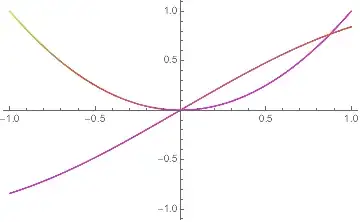
Edit for Mr. Wizard, this workaround works but involves separately finding the derivative of each function and showing the two plots together:

Show[Plot[x^2, {x, -1, 1}, ColorFunction -> Function[{x, y}, ColorData["NeonColors"][2 x]]],Plot[Sin[x], {x, -1, 1},ColorFunction -> Function[{x, y}, ColorData["NeonColors"][Cos[x]]]], PlotRange -> {-1, 1}]  

Mathematica graphics

Michael E2
  • 235,386
  • 17
  • 334
  • 747
Shaggy1135
  • 171
  • 6

2 Answers2

5

CORRECTED for scaling.

f1[x_] = x^2;
f2[x_] = Sin[x];

Show[
 Plot[f1[x], {x, -1, 1}, 
  ColorFunction -> Function[{x, y}, ColorData["DarkRainbow"][f1'[x]]]],
 Plot[f2[x], {x, -1, 1}, 
  ColorFunction -> Function[{x, y}, ColorData["DarkRainbow"][f2'[x]]]],
 PlotRange -> All]

enter image description here

However, since the the documentation states that the x values fed to ColorFunction are scaled to {0,1} the unscaled x values would be

Show[ Plot[f1[x], {x, -1, 1}, ColorFunction -> Function[{x, y}, ColorData["DarkRainbow"][f1'[2 x - 1]]]], Plot[f2[x], {x, -1, 1}, ColorFunction -> Function[{x, y}, ColorData["DarkRainbow"][f2'[2 x - 1]]]], PlotRange -> All]

enter image description here

Bob Hanlon
  • 157,611
  • 7
  • 77
  • 198
  • Isn't this what the OP says she/he wants avoid? – Michael E2 Jan 13 '15 at 21:57
  • 1
    @Michael - AFAIK ColorFunction takes only one argument so if each curve is to be colored by its derivative there needs to be two Plot calls. And I did not calculate the derivative outside of the ColorFunction which is what he wanted to avoid. – Bob Hanlon Jan 13 '15 at 22:04
  • That's pretty much the way I see how ColorFunction works, too. Since the OP seems to know how to color the individual graphs already, I figure an answer should explain why there is no other workaround. Unless there is one, of course. – Michael E2 Jan 13 '15 at 22:06
  • Couldn't you use ColorFunctionScaling -> False to get around this? – David Z Jan 13 '15 at 22:51
  • @DavidZ - that is valid approach. The one I used is somewhat shorter code. – Bob Hanlon Jan 13 '15 at 22:58
  • Yes, though if I understand correctly, the approach in this answer needs to be manually modified to match the plot range in each case. Setting ColorFunctionScaling does the same thing but with the same syntax in every case. – David Z Jan 13 '15 at 23:16
  • I hoped for an answer like those of Chip Hurst or kguler. Both seem generalizable to the extent that I won't have to individually find the derivative of each function used. Thank you for reminding me to consider ColorFunctionScaling, but showing two separate plots together is something I could already do. – Shaggy1135 Jan 14 '15 at 01:17
2

Post-processing Lines to add VertexColors that depend on the value of the derivative:

funcs = {x^2, Sin[x]};
plt = Plot[funcs, {x, -1, 1}, PlotStyle -> Thick, ImageSize -> 400];
plt2 = Block[{j = 1, k}, Normal[plt] /. Line[z_] :> 
       (k = j++; Line[z, VertexColors -> (ColorData["Rainbow"] /@ 
            ((D[funcs[[k]], x] /. x -> #) & /@ Rescale[z[[All, 1]]]))])];

Row[{plt, plt2}, Spacer[10]]

enter image description here

Update: Dealing with Plot3D following @MichaelE2's suggestion in the comments: use the VertexNormals as a basis for VertexColors:

ClearAll[dF, showF];
dF[k_: 1] := # /. HoldPattern[VertexNormals -> vn_] :>
     {VertexNormals -> vn, VertexColors -> (ColorData["Rainbow"] /@Rescale[vn[[All, k]]])} &;
showF[k_: 1] := Show[(Plot3D[#, {x, -2, 2}, {y, -2, 2},
         Mesh -> None, ImageSize -> 350, BoxRatios -> 1] // dF[k]) & /@ #,
    PlotRange -> All, Lighting -> "Neutral"] &;

Example:

funcs = {x^2 + y^2, Sin[x + y^2]};
Row[showF[#]@funcs & /@ {1, 2, 3}, Spacer[10]]

enter image description here

kglr
  • 394,356
  • 18
  • 477
  • 896
  • Ah, that's what I was going to do! :) Just couldn't get back to it.... +1 – Michael E2 Jan 14 '15 at 00:30
  • Thank you for your answer. It's a shame that Mathematica requires such a complex procedure to acquire a seemingly simple result. I can certainly use your method, but this doesn't seem generalizable to Plot3D, which would be nice. – Shaggy1135 Jan 14 '15 at 01:04
  • @Shaggy1135, good question. I think the approach suggested by Bob is more straightforward and it can be made to work for Plot3D too. – kglr Jan 14 '15 at 02:34
  • @Shaggy1135 In one way Plot3D is easier: One can use the VertexNormals as a basis for VertexColors. – Michael E2 Jan 14 '15 at 03:10
  • @MichaelE2, thank you again. – kglr Jan 14 '15 at 11:46
  • Corrected: It might be worth pointing out that the normals are normalized: vn is a list of $(−f_x,−f_y,1)/\sqrt{f_x^2+f_y^2+1}$. The gradients $(f_x, f_y)$ are given by -vn[[All, 1;;2]]/vn[[All, 3]] and so forth. (You're welcome, and sorry for the typo earlier.) – Michael E2 Jan 14 '15 at 11:48