NDSolve ensemble of initial points

Question

I want to illustrate how the differential equation depends on the initial conditions. First if all differential equations:

x'[t] == -p[t]*Cos[2*x[t]], 
p'[t] == (1 - p[t]^2)*Sin[2*x[t]]

Now, I want to put many initial conditions (x[0],p[0]) with gaussian ensemble around given point (x,p) - lets say 200 and illustrate how the position of those points changes in the plane (x,p).

Initialy it should look like this:

Ham[x_,p_]:= (1-p^2)*Cos[2*x]
ContourPlot[Ham[x,p],{x, 0, 2 Pi}, {p, -1, 1}, 
     ContourShading -> None, ContourStyle ->GrayLevel[0.1], Contours -> 20]

enter image description here

its not clear where you need help, how to solve the equations, how to plot the results, how to generate random initial points, (all of the above?) — george2079, Jan 15 '15 at 23:55
Somewhat related: http://mathematica.stackexchange.com/questions/34837/how-to-draw-the-image-of-a-circle-under-the-action-of-a-transformation-of-the-ph -- my answer could be adapted by using your ODE for the flow and your points instead of the circle of points. — Michael E2, Jan 16 '15 at 13:46

score 1 · Answer 1 · answered Jan 16 '15 at 09:14

Try the following. Here are your definitions:

 eq1 = x'[t] == -p[t]*Cos[2*x[t]]; 
eq2 = p'[t] == (1 - p[t]^2)*Sin[2*x[t]];

Ham[x_, p_] := (1 - p^2)*Cos[2*x]
pl = ContourPlot[Ham[x, p], {x, 0, 2 Pi}, {p, -1, 1}, 
   ContourShading -> None, ContourStyle -> GrayLevel[0.1], 
   Contours -> 20];

These are the list "lst" of initial points and the solution of the equations:

 lst = Transpose[{RandomReal[{0, 2 \[Pi]}, {10}], 
    RandomReal[{-1, 1}, 10]}];
sol = NDSolve[{eq1, eq2, x[0] == #[[1]], p[0] == #[[2]]}, {x, p}, {t, 
      0, 1}] & /@ lst;

This is the animation:

    Animate[
 Show[{
   pl,
   ParametricPlot[{x[t], p[t]} /. Flatten[sol, 1], {t, 0, t1}, 
     PlotTheme -> "Classic", PlotStyle -> Red] /. Line -> Arrow
   }], {t1, 0, 1}]

Should look like the following:

enter image description here

Have fun!

Pincopallino · Accepted Answer · 2015-01-16T10:35:45.157

Here is a possible solution. First, we define the final time

tf = 5;

and we generate n initial points, according to a gaussian distribution with variance sigma, centered in x0,p0.

InitialPoints = 
 With[{x0 = 0, p0 = 0, sigma = .3, n = 10}, 
  Transpose[{RandomVariate[NormalDistribution[x0, sigma], n], 
   RandomVariate[NormalDistribution[p0, sigma], n]}]]

The result is a list of n pairs of coordinates.

Then we solve the differential equations for each given initial point

s = NDSolve[{x'[t] == -p[t]*Cos[2*x[t]], 
  p'[t] == (1 - p[t]^2)*Sin[2*x[t]], x[0] == #[[1]], 
  p[0] == #[[2]]}, {x[t], p[t]}, {t, 0, 5}] & /@ InitialPoints

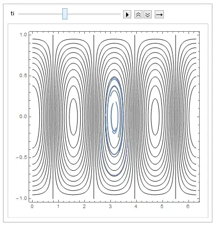
The phase space plot (your code)

Ham[x_, p_] := (1 - p^2)*Cos[2*x]
cont = ContourPlot[Ham[x, p], {x, 0, 2 Pi}, {p, -1, 1}, 
   ContourShading -> None, ContourStyle -> GrayLevel[0.1], 
   Contours -> 20];

And the animated trajectories:

Animate[Show[cont, ParametricPlot[{x[t], p[t]} /. s, {t, 0, ti}]], {ti, 0, tf}]

The result is

enter image description here

EDIT

To obtain the points at a specific time instant ti, you can use

Flatten[{x[t], p[t]} /. s /. t -> ti, 1]

to obtain a list of pairs of coordinates, and

Show[cont, Graphics[Point[Flatten[{x[t], p[t]} /. s /. t -> ti, 1]]]]

to obtain a plot like

enter image description here

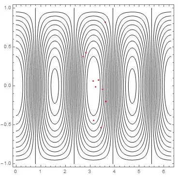
Of course you can change the point style to suit your needs. You can also animate the plot, or show initial and final points with different colors.

Thank You very much for Your nice reponse :) but I want to have a group of dots on the picture, not lines - You start with a group of dots scattered around given point and then in some time $t$ You have this group in different place according to equations of motion. It doesn't have to an animation at the end. I just want a "photo" of this group - position of all dots in different moments of time. It has to look like a scatter plot — WoofDoggy, Jan 16 '15 at 10:21

NDSolve ensemble of initial points

2 Answers2

Linked