2

I have a dataset (of DNA reads corresponding to the human mitochondrial DNA) which I want to plot on a polar plot, with the distance corresponding to the G-C percentage of the DNA in that segment.

The raw data to generate the plot is:

plotArr = {{1, 1380, 1512, 48}, {2, 2501, 2687, 47}, {3, 15205, 15514, 47}, {4, 
  1390, 1129, 49}, {5, 5313, 5523, 42}, {6, 12948, 13165, 53}, {7, 
  14401, 14044, 43}, {8, 2207, 2525, 39}, {9, 7875, 8463, 44}, {10, 
  15528, 15943, 43}, {11, 9943, 9391, 46}, {12, 6238, 5515, 46}, {13, 
  16570, 15949, 45}, {13, 299, 1, 45}, {14, 1500, 2191, 41}, {15, 318,
   1143, 46}, {15, 276, 302, 46}, {16, 14392, 15217, 45}, {17, 13194, 
  14063, 46}, {18, 8430, 9408, 44}, {19, 11679, 12959, 43}, {20, 6208,
   7859, 45}, {21, 11681, 9918, 41}, {22, 5317, 3591, 45}, {22, 3566, 
  2667, 45}, {99, 0, 16570, 45.5}}

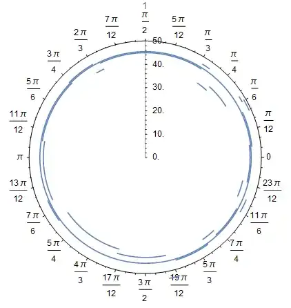
I then use a Show function to independently plot all of the DNA segments as arcs on the polar plot. This plots them correctly.

  Show[Table[
  PolarPlot[{plotArr[[i]][[4]]}, {t, plotArr[[i]][[2]]*Pi*2/16570, 
    plotArr[[i]][[3]]*Pi*2/16570}, PlotLabel -> plotArr[[i]][[1]]]
  , {i, Length[plotArr]}]]

enter image description here

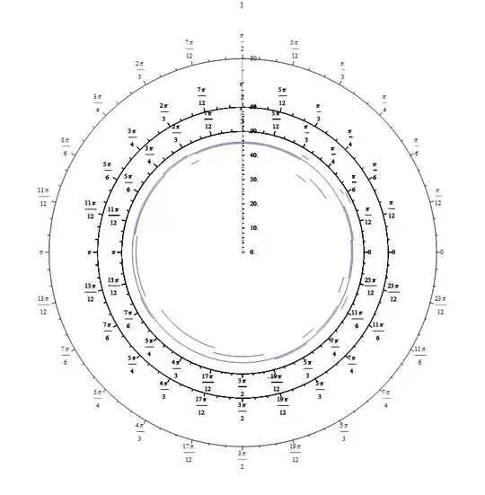
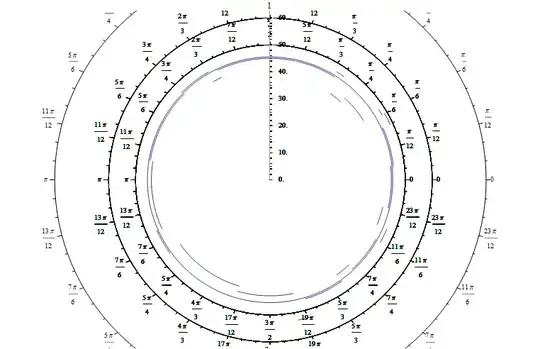
However, adding the option PolarAxes->True completely messes the graph up.

enter image description here

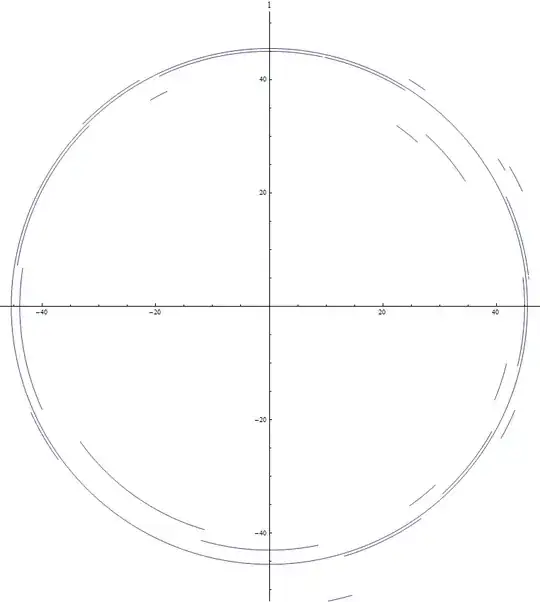
Adding PlotRange -> {-50, 50} doesn't help, it changes the graph to this instead.

enter image description here

How do I correctly do this plot, so that it has a PolarAxes, and also a unified distance axis?

Also, what would be the best way to go about labelling each arc with its own label? (I attempted PlotLabel, but that only works for the entire plot)

March Ho
  • 649
  • 5
  • 15

4 Answers4

5

you can try this also:

 plotArr = Sort[plotArr, #1[[4]] > #2[[4]] &];
    lable = Table[
       Text[Style[plotArr[[i]][[1]], Red, Bold], 
        plotArr[[i]][[4]] {Cos[#], Sin[#]} &@
         Mean[{plotArr[[i]][[2]]*Pi*2/16570, 
           plotArr[[i]][[3]]*Pi*2/16570}]], {i, 1, Length[plotArr]}];
    Show[Table[
       PolarPlot[{plotArr[[i]][[4]]}, {t, plotArr[[i]][[2]]*Pi*2/16570, 
         plotArr[[i]][[3]]*Pi*2/16570}, PolarAxes -> (i == 1), 
        Epilog -> 
         Text[Style[plotArr[[i]][[1]], Red, Bold, 16], 
          plotArr[[i]][[4]] {Cos[#], Sin[#]} &@
           Mean[{plotArr[[i]][[2]]*Pi*2/16570, 
             plotArr[[i]][[3]]*Pi*2/16570}]]], {i, 1, 
        Length[plotArr]}]] /. Rule[Epilog, _] :> Rule[Epilog, lable]

enter image description here

Basheer Algohi
  • 19,917
  • 1
  • 31
  • 78
3

I am not entirely sure I understand what you want but perhaps using PolarAxes -> (i == 1) does it?

Table[PolarPlot[{plotArr[[i]][[4]]}, {t, plotArr[[i]][[2]]*Pi*2/16570, 
    plotArr[[i]][[3]]*Pi*2/16570}, PlotLabel -> plotArr[[i]][[1]], 
   PolarAxes -> (i == 1)], {i, Length[plotArr]}] // Show

enter image description here

Mr.Wizard
  • 271,378
  • 34
  • 587
  • 1,371
  • Ah, that's great. What about the other part of the question (labelling the arcs independently) though? – March Ho Jan 22 '15 at 20:13
  • @March Where should the labels be? There are so many segments that I have trouble imagining them all fitting. Would Tooltips be useful? – Mr.Wizard Jan 22 '15 at 20:16
  • The image is supposed to be exported, and not viewed within Mathematica, so I don't think Tooltips will help. There are only ~20 or so segments though, so I don't think that's too many? – March Ho Jan 22 '15 at 20:17
  • @March Okay. I am not trying to be obstinate but I still have trouble imagining it. Would you be willing to manually draw labels for this one plot to illustrate what you would like? I would then attempt to programmatically recreate it for application to other, similar plots. – Mr.Wizard Jan 22 '15 at 20:18
  • @March What about coloring each segment uniquely and then using a legend? – Mr.Wizard Jan 22 '15 at 20:19
  • I think colouring them will not be a good idea due to the large number of segments making it difficult to distinguish the colours. Could you just point me to the relevant labelling function for labelling a part of a line graph? – March Ho Jan 22 '15 at 20:21
  • I think it might be especially bad on your side since your image is rather small, I intend to export this image on a much larger scale, so I think labelling is a reasonable option. – March Ho Jan 22 '15 at 20:23
  • 1
    Actually Algohi has provided the answer, that was exactly what I had in mind. – March Ho Jan 22 '15 at 20:24
3

Although I understand the rationale for not wishing to distinguish curves by color, the approach below may be of interest to others.

plotscl = MapAt[N[# Pi*2/16570] &, plotArr, {{All, 3}, {All, 2}}];
Show[PolarPlot[Evaluate[Table[Piecewise[{{plotArr[[i, 4]], 
  Min[plotscl[[i, 2]], plotscl[[i, 3]]] < t < Max[plotscl[[i, 2]], plotscl[[i, 3]]]}}, I],
  {i, Length[plotArr]}]], {t, 0, 2 Pi}, PlotRange -> 50, PlotPoints -> 100, 
  PlotLegends -> Cases[plotArr, {z_, _, _, _} -> z]], 
  PolarPlot[40, {t, 0, .0000001}, PlotRange -> 20, PolarAxes -> True], ImagePadding -> 50, 
  PlotRangeClipping -> False, ImageSize -> 500]

color plot

bbgodfrey
  • 61,439
  • 17
  • 89
  • 156
1

Rescale columns 2 and 3 to the interval (0, 2 Pi):

{min, max} = Through@{Min, Max}@plotArr[[All, {2, 3}]];
(* {0, 16570} *)
data = MapAt[N[ Rescale[#, {min, max}, {0, 2 Pi}]] &, plotArr, {All, {2, 3}}];

Define two helper functions to be Applyed to data to produce the polar plots and the text labels:

ClearAll[ppF, epilogF]
ppF[opts : OptionsPattern[PolarPlot]] := PolarPlot[{#4}, {t, #2, #3}, opts] &;
epilogF = Module[{m = Mean[{#2, #3}]}, Text[Style[#, Red, 16, Bold], #4 {Cos[m], Sin[m]}]] &;

Create an empty polar plot with the desired polar axes specification:

emptypp = PolarPlot[1, {t, 0, 2 Pi}, PlotStyle->None, Axes->False, BaseStyle->(FontSize->16),
                    PolarAxes -> True, PolarAxesOrigin -> {Pi/2, 60}];

Apply (@@@) ppF to rescaled data and overlay with emptypp using Show and setting Epilog option value to epilogF@@@data:

Show[emptypp, ppF[PlotStyle -> Dynamic[{Hue[RandomReal[]], Thick}]] @@@ data,
     ImageSize -> 600, Epilog -> (epilogF @@@ data)]

enter image description here

Update: You can also add the text labels using Mesh:

ClearAll[ppF2, meshF]
meshF[col_: Red, fsize_: 14, fweight_: Plain, ffamily_: "Arial"] := 
  Module[{m = Mean[{#2, #3}]}, 
        {{{Mean[{#2, #3}], 
           {col,PointSize[0], 
            FontSize -> fsize, FontWeight -> fweight, FontFamily -> ffamily,  
            Text[#, #4 {Cos[m], Sin[m]}]}}}}] &;

ppF2[opts:OptionsPattern[PolarPlot]] := PolarPlot[{#4}, {t, #2, #3}, opts, Mesh->(meshF[][##])] &;

Show[emptypp, ppF2[] @@@ data, Axes -> False, ImageSize -> 400]

enter image description here

kglr
  • 394,356
  • 18
  • 477
  • 896
  • If I need Matlab Type of Plots (https://de.mathworks.com/help/matlab/ref/polarplot.html), how to set the parameters – ABCDEMMM Oct 13 '18 at 23:23
  • @ABCDEMMM, see PolarPlot. E.g. PolarPlot[Sin[4 t], {t, 0, 2 Pi}] – kglr Oct 13 '18 at 23:27
  • PolarPlot[yy, {x, 0, 2*Pi}, PolarAxes -> True, PolarTicks -> {"Degrees", Automatic}, PolarGridLines -> True, Mesh -> 15, MeshStyle -> Directive[PointSize[Large], Red]] I have done, thanks. – ABCDEMMM Oct 13 '18 at 23:30