I just realized that the parametrization in my previous revision of this answer is a special case of bipolar coordinates. Every rectangle in bipolar coordinates $\theta_1<\theta<\theta_2,\ \tau_1<\tau<\tau_2$ is a region between four arcs. Two arcs is just a simple special case.
Here is my realization of bipolar coordinates with special stretching to make texture more uniform and avoid shrinking at points $\tau=\pm\infty$. This parametrization have two additional parameters $(\theta_0,\tau_0)$. It is a reference point where texture is locally uniform.
bc[{τ1_, τ2_, τ0_: 1}, {θ1_, θ2_, θ0_: Scaled[0.5]}, opts___] :=
 Module[{u, v, t, q, t1, t2, q1, q2, μ, ν},
  μ = Abs@Tan[θ0/2] /. Scaled@x_ :> Rescale[x, {0, 1}, {θ1, θ2}] // Chop;
  ν = Abs@Tanh[τ0/2] /. Scaled@x_ :> Rescale[x, {0, 1}, {τ1, τ2}] // Chop;
  {t1, t2} = Which[μ == 0, #, Chop[1/μ] == 0, -1/#, True, ArcTan[# μ]] &@Tanh[{τ1, τ2}/2];
  {q1, q2} = If[ν == 0, Tan[#/2], ArcTan[ν+1 - Cos@#(ν-1), Sin@#(ν-1)] + #/2] & /@ {θ1, θ2};
  u = Which[μ == 0, t, Chop[1/μ] == 0, -1/t, True, Tan@t/μ];
  v = If[ν == 0, q, Tan@q/ν];
  First@Cases[#, _GraphicsComplex, ∞] &@
   ParametricPlot[{u (1 + v^2), (1 - u^2) v}/(1 + u^2 v^2), {t, t1, t2}, {q, q1, q2}, opts]]
You can use any option of the parametric plot
Graphics[bc[{0.5, 4}, {-π, π/2}, Mesh -> Full, PlotStyle -> {Opacity[1],
    Texture@LinearGradientImage[{Red, Yellow, Blue}]}, BoundaryStyle -> Black]]

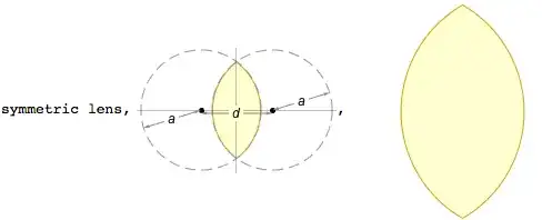
As mentioned above, two arcs is a special case
arcs[p1_, r1_, p2_, r2_, opts___] :=
 Module[{α = ArcTan @@ (p1 - p2), d = Norm[p2 - p1], a, τ1, τ2, d2},
  d2 = (d^2 + r1^2 - r2^2)/(2 d); a = Sqrt[d2^2 - r1^2];
  τ1 = Log[-(d2 + a)/r1]; τ2 = Log[(d2 + a - d)/r2];
  GeometricTransformation[#2, {Abs@a {{Cos@α, -Sin@α}, {Sin@α,
         Cos@α}}, #}] &[p2 - {Cos@α, Sin@α} a Coth[τ2],
   If[Im@a == 0, bc[{τ1, τ2}, {0, 2 π, π/2}, opts], α += π/2;
    bc[{-∞, ∞}, {Im@τ1, Im@τ2}, opts]]]
  ]

p1 = {0.6, 0.2};
p2 = {0.9, 0.6};
r1 = 0.5;
r2 = 0.7;
Graphics[arcs[p1, -r1, p2, r2, PlotStyle -> {Opacity[1],
    Texture@LinearGradientImage[{Top, Bottom} -> {Red, Yellow,
        Blue}]}, BoundaryStyle -> Black]]

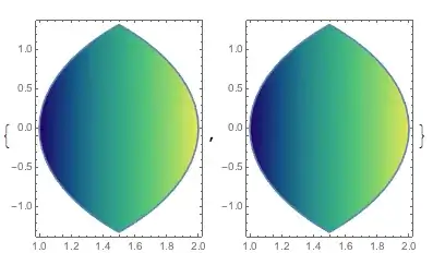
The output region (intersection, complement or union) depends on signs of radii
Graphics[arcs[p1, r1, p2, r2, PlotStyle -> {Opacity[1],
    Texture@LinearGradientImage[{Top, Bottom} -> {Red, Yellow,
        Blue}]}, BoundaryStyle -> Black]]

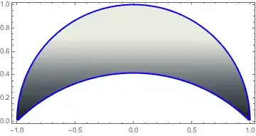
In the current realization the intersection of initial circles is not necessary
p1 = {2.5, 0.2};
p2 = {0.9, 0.6};
r1 = -3.5;
r2 = 0.7;
Graphics[{arcs[p1, r1, p2, r2, PlotStyle -> {Opacity[1],
     Texture@LinearGradientImage[{Red, Yellow, Blue}]},
   BoundaryStyle -> Black]}]

You can do even open regions (here RegionFunction limits the region)
p1 = {0.5, 0.2};
p2 = {-1.1, 0.6};
r1 = -0.5;
r2 = -0.7;
Graphics[arcs[p1, r1, p2, r2, Mesh -> Full, PlotStyle -> {Opacity[1],
    Texture@LinearGradientImage[{Red, Yellow, Blue}]},
  BoundaryStyle -> Black, RegionFunction -> Function[{x, y}, x^2 + y^2 < 200],
  MaxRecursion -> 3], PlotRange -> 4]