Making table and plotting results of NDSolve problem

Question

I am trying to solve two equation to find /[Phi][x] and plot h vs. /[Phi][x] for different values of L.I tried by writing as:

sol[h_, L_] := NDSolve[{f''[x] == f[x] (Φ'[x])^2 - f[x] (1 - f[x]^2), 
  h - (f[x])^2 Φ'[x] == 0., Φ[0.] == 0., 
  f[0.] == f[L] == 1.}, {Φ}, {x, 0, L}, Method -> {"Shooting", 
 "StartingInitialConditions" -> {f[0] == 1, 
  f'[0] == 0, Φ[0.] == 0.}, MaxIterations -> 100}]
t3 = Table[{sol[h, L], h}, {h, 0, 1}, {L, 1, 8}]
ListPlot[Evaluate[t3]]

But it's not giving any plot. Can anyone please help me.

---

Thanks @Alexei Boulbitch for your help. But you have plotted f[x] with x, but I'm looking for h vs. ϕ[x]. You're absolutely correct that there are some restrictions on the value of h. The range of h will be controlled by the the condition that f[L]=1. So to see the range of h for different values of L I've coded the following :

Manipulate[sols = 
  NDSolve[{f''[x] == h^2/f[x]^3 - f[x] (1 - f[x]^2), f[0] == f[L] == 1}, f[x], x, 
   Method -> {"Shooting", "StartingInitialConditions" -> {f[0] == 1, f'[0] == 0}, 
     MaxIterations -> 100}];
 Plot[Evaluate[{f[x]} /. sols], {x, 0, L}, PlotRange -> {0, 1}], {{h, .7, "cureent"}, 
  0, .99}, {{L, 1, "length"}, 1, 8}]

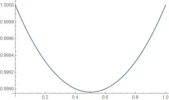
This gives out the following-

Now with this in my hand I can Plot h vs. ϕ[x] . To do that I'm doing the following

t1 = Table[{h, 
    NDSolve[{f''[x] - h^2/f[x]^3 + f[x] (1 - f[x]^2) == 0, f[0.] == f[1.] == 1.}, 
     f[x], {x, 0, 1}, 
     Method -> {"Shooting", "StartingInitialConditions" -> {f[0] == 1, f'[0] == 0}, 
       MaxIterations -> 100}]}, {h, 0, .98, .01}];

t2 = Table[{Evaluate[ϕ[x] /. 
      NDSolve[{t1[[n]][[1]] - (Evaluate[f[x] /. t1[[n]][[2]]])^2 ϕ'[x] == 
         0, ϕ[0.] == 0}, ϕ[x], {x, 0, 1}]], t1[[n]][[1]]}, {n, 1, 99}];

ListPlot[table2]

But, unfortunately this is not working . I've also tried with ParametricNDSolve, again there was some similar problems. Could you please help me getting the plot I'm

Answer 1

You should take the second equation, express Φ'[x]from it and substitute into the first one:

Clear[h, L];
f''[x] == 
  f[x] (Φ'[x])^2 - 
   f[x] (1 - f[x]^2) /. (Solve[
    h - (f[x])^2 Φ'[x] == 0, Φ'[x]][[1, 1]])

(*  f''[x] == h^2/f[x]^3 - f[x] (1 - f[x]^2)  *)

Then you may solve the obtained equation, say, as follows:

L = 1;
h = 0.1;
s = NDSolve[{f''[x] == 
     h^2/f[x]^3 - f[x] (1 - f[x]^2), f[0] == 1, f[L] == 1}, 
   f, {x, 0, L}][[1, 1]]
Plot[f[x] /. s, {x, 0, L}]

This returns the following plot:

Playing with this code shows that with increasing h one sooner or later falls into divergence. So, I would think that there are some limitations on the values of parameters, particularly, h.

Have fun!