PredictionBands and the presence of {0,0} point

Question

We know from this post, that the default fitting method cannot handle data with a {0,0} point, and that there are alternative methods.

But, with these alternative methods, the prediction bands property fails.

How to solve this?

newData = Table[{q, 2*q^2*RandomReal[{0.80, 1.2}]}, {q, 0, 2, 0.01}];
newModel = NonlinearModelFit[newData, a*q^b, {a, b}, q, Method -> "PrincipalAxis"];
Show[ListPlot[newData], Plot[newModel["SinglePredictionBands", ConfidenceLevel -> 0.95], {q, 0, 2}]]

(* FittedModel::nodm: Unable to compute an approximate design matrix because derivatives of the model could not be found. Some property values cannot be computed. *)

Chris Degnen · Answer 1 · 2015-02-17T21:39:31.333

There doesn't seem to be so much a problem with the fitting method. Your model is actually linear, but values of zero are problematic for it.

Quoting from J. Johnston's Econometric Methods, edition 3, page 13:

A linear specification means that Y, or some transformation of Y, can be expressed as a linear function of X, or some transformation of X. In this sense,

Y = α + βX

Y = αX^β

and Y = exp{α + β 1/X}

are all linear specifications. The first is already linear in Y and X. The second, on taking logarithms of both sides of the equation, may be written as

log Y = log α + β log X

which is linear in log Y and log X.

To get around the problem of Log[0.] why not introduce small values?

E.g. comparing methods, first with the {0., 0.} point included:

newData = Table[{q, 2*q^2*RandomReal[{0.80, 1.2}]}, {q, 0, 2, 0.01}];
newModel = NonlinearModelFit[newData, a*q^b, {a, b}, q, Method -> "PrincipalAxis"];
Normal[newModel]

1.9184111799203873 q^2.1104032823834475

newData[[1]]

{0., 0.}

Setting small values:

newData[[1]] = {1.*^-100, 1.*^-100};
newModel2 = NonlinearModelFit[newData, a*q^b, {a, b}, q];
Normal[newModel2]

1.9184111852020502 q^2.110403278099661

The results are not much different.

Furthermore, upon checking, Method -> "PrincipalAxis" doesn't actually help for this model:

With the small values included the "PrincipalAxis" method gives the same result as before (when the zeros were used), indicating that it is less precise than the default method.

newModel = NonlinearModelFit[newData, a*q^b, {a, b}, q, Method -> "PrincipalAxis"];
Normal[newModel]

1.9184111799203873 q^2.1104032823834475

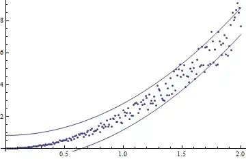
Plotting the bands with the default method (and small values replacing zeros):

Show[ListPlot[newData], Plot[newModel2["SinglePredictionBands",
   ConfidenceLevel -> 0.95], {q, 0, 2}]]

enter image description here

score 3 · Answer 2 · answered Feb 17 '15 at 21:41

If the data and the error follows a power law, it makes sense to do the fit in log log space. To do that I'm dropping zero/negative data:

newData = 
     Select[ Table[{q, 2*q^2*RandomReal[{0.80, 1.2}]}, {q, 0, 2, 0.01}] , 
        #[[1]] > 0 && #[[2]] > 0 &] ;
newModel = 
     NonlinearModelFit[Log[newData], a*q + b, {a, b}, q, Method -> "PrincipalAxis"];
Show[{
        ListPlot[newData],
        Plot[ Exp[newModel[Log[q]]] , {q, .1, 2}],
        Plot[ Exp[ 
          newModel["SinglePredictionBands", ConfidenceLevel -> 0.95] ]  /. 
             q -> Log[lq] , {lq, .1, 2}]}]

enter image description here

for comparison, your model with the exact zero dropped from the data looks like this:

enter image description here

PredictionBands and the presence of {0,0} point

2 Answers2