Here is a way to do it:
TruncatedOctahedron =
  ImplicitRegion[{x + y + z <= 10 && x + y - z <= 10 &&
     x - y + z <= 10 && -x + y + z <= 10 && x + y + z >= -10 &&
     x + y - z >= -10 &&
     x - y + z >= -10 && -x + y + z >= -10 && -6 <= x <= 6 && -6 <=
      y <= 6 && -6 <= z <= 6}, {x, y, z}];
We use exact faces to construct the boundary element mesh. For this we first make a boundary element mesh from this:
Needs["PolyhedronOperations`"]
gc = Truncate[PolyhedronData["Octahedron", "Faces"], 4/10];
gc[[1]] *= 14.14213;
dg = DiscretizeGraphics[gc];
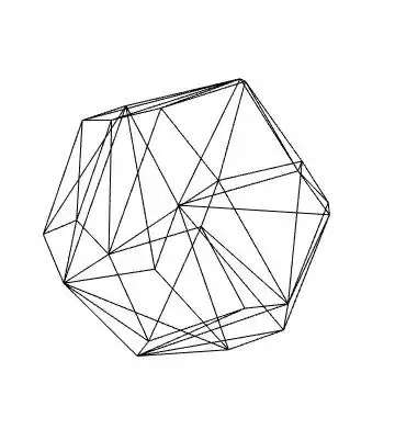
(to = ToBoundaryMesh[dg])["Wireframe"]
Next, we create the boundary element mesh and check that the truncated octahedron is matches to one you posted:
Needs["NDSolve`FEM`"]
cl = 100;
bmesh = ToBoundaryMesh[
"Coordinates" ->
Join[to["Coordinates"],
cl*{{-1., -1., -1.}, {1., -1., -1.}, {1., 1., -1.},
{-1., 1., -1.}, {-1., -1., 1.}, {1., -1., 1.}, {1., 1.,
1.}, {-1., 1., 1.}}],
"BoundaryElements" ->
Join[to["BoundaryElements"], {QuadElement[
Length[to["Coordinates"]] + {{1, 2, 3, 4}, {8, 7, 6, 5}, {1,
5, 6,
2}, {2, 6, 7, 3}, {3, 7, 8, 4}, {4, 8, 5, 1}}]}],
"RegionHoles" -> {{0, 0, 0}}];
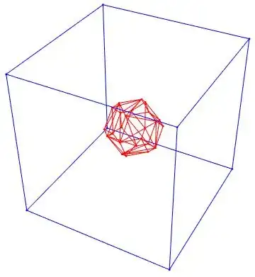
Show[
RegionPlot3D[TruncatedOctahedron],
bmesh["Wireframe"], "PlotRange" -> {{-10, 10}, {-10, 10}, {-10, 10}}
]

In a next step we add markers to the boundary mesh. Once the full mesh is generated those will be propagated and we can use them from within NDSolve.
pointMarkerFunction = Compile[{{coords, _Real, 2}},
   Which[
      Sqrt[Total[#^2]] <= 10, 1,
      True, 2] & /@ coords];
boundaryMarkerFunction =
  Compile[{{boundaryElementCoords, _Real,
     3}, {pointMarkres, _Integer, 2}},
   Which[
      Union[#] === {1}, 1,
      True, 2 ] & /@ pointMarkres];
cl = 20; (* made this a bit smaller *)
bmesh = ToBoundaryMesh[
   "Coordinates" ->
    Join[to["Coordinates"],
     cl*{{-1., -1., -1.}, {1., -1., -1.}, {1., 1., -1.},
       {-1., 1., -1.}, {-1., -1., 1.}, {1., -1., 1.}, {1., 1.,
        1.}, {-1., 1., 1.}}],
   "BoundaryElements" ->
    Join[to["BoundaryElements"], {QuadElement[
       Length[to["Coordinates"]] + {{1, 2, 3, 4}, {8, 7, 6, 5}, {1,
          5, 6,
             2}, {2, 6, 7, 3}, {3, 7, 8, 4}, {4, 8, 5, 1}}]}],
   "RegionHoles" -> {{0, 0, 0}},
   "PointMarkerFunction" -> pointMarkerFunction,
   "BoundaryMarkerFunction" -> boundaryMarkerFunction];
We inspect the point and boundary markers:
Show[
 bmesh["Wireframe"[Boxed -> False,
   "MeshElementStyle" -> {EdgeForm[Red], EdgeForm[Blue]}]],
 bmesh["Wireframe"[Boxed -> False, "MeshElement" -> "PointElements",
   "MeshElementStyle" -> {Red, Blue}]]
 ]
Create the mesh:
mesh = ToElementMesh[bmesh]
Solve the PDE:
sol = NDSolveValue[{Laplacian[u[x, y, z], {x, y, z}] ==
    0, {DirichletCondition[u[x, y, z] == 200., ElementMarker == 1],
    DirichletCondition[u[x, y, z] == 15., ElementMarker == 2]}},
  u, {x, y, z} \[Element] mesh]
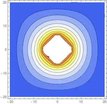
Visualize the solution:
Manipulate[
 ContourPlot[sol[x, y, z], {x, -cl, cl}, {y, -cl, cl},
  RegionFunction ->
   Function[{x, y}, ElementMeshRegionMember[mesh, {x, y, z}]],
  ColorFunction -> "TemperatureMap",
  Contours -> Range[15, 200, (200 - 15)/10.]], {{z, 0}, -cl, cl, 1}]
More details about the mesh generation and visualization can be found here, here, here and here
TruncatedOctahedronSet (=)must stay instead of==and the semicolumn ";" should stay after the curly brace. – Alexei Boulbitch Mar 13 '15 at 08:40