9

The Doolittle Decomposition algorithm as below: $$A=LU$$ where

$A= \begin{pmatrix} a_{11} & a_{12} & \cdots a_{1n}\\ a_{21} & a_{22} & \cdots a_{2n}\\ \vdots & \vdots & \vdots \\ a_{n1} & a_{n2} & \cdots a_{nn}\\ \end{pmatrix} L=\begin{pmatrix} 1 & 0 & \cdots 0\\ l_{21} & 1 & \cdots 0\\ \vdots & \vdots & \vdots \\ l_{n1} & l_{n2} & \cdots 1\\ \end{pmatrix} $ $ U=\begin{pmatrix} u_{11} & u_{12} & \cdots u_{1n}\\ 0 & u_{12} & \cdots u_{12}\\ \vdots & \vdots & \vdots \\ 0 & 0 & \cdots u_{nn}\\ \end{pmatrix} $

And

\begin{equation} \begin{cases} u_{kj}=a_{kj}-\sum_{m=1}^{k-1}l_{km}u_{mj} && (j=k,k+1,\cdots,n)\\ l_{ik}=1/u_{kk} (a_{ik}-\sum_{m=1}^{k-1}l_{im}u_{mk}) && (i=k+1,k+2,\cdots,n) \end{cases} \end{equation}

Where, $k=1,2,\cdots,n$

Implementation

oneStep[mat_?MatrixQ, {intermediate_, index_}] :=
 Module[{temp = intermediate, k = index, row},
  row = Length@mat;
  Table[
   temp[[k, j]] =
    mat[[k, j]] - Sum[temp[[k, m]] temp[[m, j]], {m, 1, k - 1}], {j, k, row}];
  Table[
   temp[[i, k]] =
    1/temp[[k, k]] (mat[[i, k]] - 
   Sum[temp[[i, m]] temp[[m, k]], {m, 1, k - 1}]), {i, k + 1, row}];
 {temp, k+1}
]
 (*==============================*)

doolittleDecomposite[mat_?MatrixQ] :=
 Module[{intermediate, row},
  intermediate = ConstantArray[0, Dimensions@mat];
  row = Length@mat;
  First@
   Nest[oneStep[mat, #] &, {intermediate, 1}, row]
]

Test

test={{1, 6, 1, 9}, {4, 4, 9, 7}, {10, 4, 10, 2}, {10, 3, 10, 2}};
doolittleDecomposite[test]

$\left( \begin{array}{cccc} 1 & 6 & 1 & 9 \\ 4 & -20 & 5 & -29 \\ 10 & \frac{14}{5} & -14 & -\frac{34}{5} \\ 10 & \frac{57}{20} & \frac{57}{56} & \frac{11}{7} \\ \end{array} \right)$

Namely,

$L=\left( \begin{array}{cccc} 1 & 0 & 0 & 0 \\ 4 & 1 & 0 & 0 \\ 10 & \frac{14}{5} & 1 & 0 \\ 10 & \frac{57}{20} & \frac{57}{56} & 1 \\ \end{array} \right) U=\left( \begin{array}{cccc} 1 & 6 & 1 & 9 \\ 0 & -20 & 5 & -29 \\ 0 & 0 & -14 & -\frac{34}{5} \\ 0 & 0 & 0 & \frac{11}{7} \\ \end{array} \right)$

Performance testing

SeedRandom[1234];
testReal = RandomReal[{1., 100.}, {200, 200}];
doolittleDecomposite[testReal]; // AbsoluteTiming
LUDecomposition[testReal]; // AbsoluteTiming
{6.102349, Null}
{0.034002, Null}  (*big performance difference*)
SeedRandom[12]
testInteger = RandomInteger[{1, 100}, {100, 100}];
doolittleDecomposite[testInteger]; // AbsoluteTiming
LUDecomposition[testInteger]; // AbsoluteTiming
{6.173353, Null}
{4.481256, Null}  (*a bit difference*)

Question

  • Is it possible to speed up my implementation code?
  • Could someone give me some hints(like how to organize the data) to implement this algorithm elegantly in Mathematica?Namely, I think my method is not good:)
J. M.'s missing motivation
  • 124,525
  • 11
  • 401
  • 574
xyz
  • 605
  • 4
  • 38
  • 117
  • 2
    Might try changing the sums to dot products. Also Table probably should be Do. For the machine real case you could run it through Compile. – Daniel Lichtblau Mar 31 '15 at 16:05
  • The oneStep function that I implemented is C-style(like procedural paradigm) . So my main difficult is how to store and organize the intermediate result in right way if I'd like to implement this algorithm with functional or rule-based paradigm. – xyz Apr 03 '15 at 05:21
  • Might want to check the notebook here. Dated a bit but still quite relevant to the question at hand. – Daniel Lichtblau Apr 04 '15 at 13:20
  • I've just seen this. I believe you know, but just to remind, algorithms of this sort are usually made with a pivoting strategy in place (e.g. partial, total, or rook); otherwise, there are a lot of nonsingular matrices that do not have a decomposition. – J. M.'s missing motivation Oct 24 '15 at 10:56
  • @J.M. I cannot understand the conception of pivoting strategy. Could you give a explonation about it? Or you give a counter example that is non-singular , but does not have a decomposition by the algorithm of mine – xyz Oct 24 '15 at 11:24
  • 1
    With respect to the counterexample, try Reverse[IdentityMatrix[4]]. As for pivoting: did you notice the difference between your method and LUDecomposition[]? The latter one outputs a permutation list, which encodes the (partial) pivoting (interchanges of rows) done in the course of decomposing the matrix. Any robust implementation has to have a pivoting strategy like that. – J. M.'s missing motivation Oct 24 '15 at 11:55
  • @J.M. You are right, Reverse[IdentityMatrix[4]] // doolittleDecomposite2 in this answer gives the Power::infy error information. And I noticed the difference that LUDecomposition returns a list of three elements. – xyz Oct 24 '15 at 12:31
  • @J.M. In addition, the formula that I used to implement theLU decomposition came from my textbook of Numerical Analysis. – xyz Oct 24 '15 at 12:39
  • ...and that book ought to have mentioned permutations/pivoting somewhere. – J. M.'s missing motivation Oct 24 '15 at 13:00

3 Answers3

11

It's pretty clear that the complexity of this function is $\text{O}(n^3)$, since we're iterating over each element of a matrix (a factor of $n^2$) and taking a sum at each one (an additional factor of $n$). However, we can't really do anything to reduce the complexity; LU decomposition has the same complexity as matrix multiplication. Although algorithms faster than $\text{O}(n^3)$ do exist I do not think they are used in practice.


The upshot of all this is that if we really want to increase our speed, we should Compile our function. Here is an algorithm in Fortran that is in-place; that is, it doesn't use any extra memory (although we do need to copy the matrix once so that we can 'edit' it). We can write a CompiledFunction to implement this version of the algorithm:

doolittleDecomposition = Compile[{{a, _Real, 2}},
  With[{n = Length[a]},
   Module[{t = a},
    Do[
     Do[
      Do[
        t[[i, j]] -= t[[i, k]] t[[k, j]];,
        {k, 1, i - 1}];,
      {j, i, n}];
     Do[
      Do[
       t[[j, i]] -= t[[j, k]] t[[k, i]];,
       {k, 1, i - 1}];
      t[[j, i]] /= t[[i, i]];,
      {j, i + 1, n}];,
     {i, 1, n}];
    t
    ]
   ],
  {{q, _Real}}
  , RuntimeOptions -> {"Speed", "EvaluateSymbolically" -> False}, 
  CompilationTarget -> "C", 
  CompilationOptions -> {"ExpressionOptimization" -> True}]

We should double-check that our function doesn't call MainEvaluate, which is slow:

Needs["CompiledFunctionTools`"]
doolittleDecomposition // CompilePrint

While doing this check I discovered that I originally wrote t[j, i] instead of t[[j, i]], causing MainEvaluate to be called. Always double-check! In fact, let's now double-check that both algorithms give the same result:

testReal = RandomReal[1, {200, 200}];
d1 = doolittleDecomposite[testReal]; // AbsoluteTiming
d2 = doolittleDecomposition[testReal]; // AbsoluteTiming
d1 == d2

This also shows that the Compiled version is faster.

Update: Refactoring the original code

If you think Compile is too drastic (or you don't have a working C compiler) there are some other changes we can make.

  • Don't use an auxiliary or 'helper' function. This will incur extra overhead that you don't need. Unlike a compiled language where the compiler will essentially inline the function, Mathematica will be passing-by-value all of your matrices!
  • Don't use Nest. If we're getting rid of the helper function, Nest doesn't really make sense. We can replace it with a Do-loop instead. The Do-loop can 'automatically' increment k, instead of having to pass it (in a list!) to a function and have it returned (also in a list!!). At this point we can rename intermediate to temp, consolidating two variables that really contain the same thing, and we also can lose the extra redefinition of row inside the loop.
  • Use Dot instead of Sum. In general, if there's a builtin function for something, that function is faster. In this case you want to pairwise multiply two lists and take the sum of the resulting elements. We usually call that a dot product. Instead of looping m, we can use Span to extract a list using Part, and then Dot our two lists together. This is where most of the speedup comes from.

At this point the code looks pretty much like the Fortran function, but with the inner loops handled by Dot:

doolittleDecomposite2[mat_?MatrixQ] := 
 Module[{temp = ConstantArray[0, Dimensions@mat], row = Length@mat},
  Do[
   Do[temp[[k, j]] =
     mat[[k, j]] - temp[[k, ;; k - 1]].temp[[;; k - 1, j]],
    {j, k, row}];
   Do[temp[[i, k]] =
     (mat[[i, k]] - temp[[i, ;; k - 1]].temp[[;; k - 1, k]]) / temp[[k, k]],
    {i, k + 1, row}];,
   {k, row}];
  temp
  ]

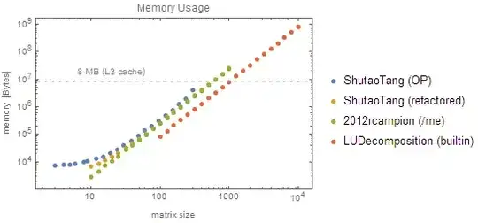
Updated performance analysis

I ran another comparison, this time including LUDecomposition, just to see how well we did:

enter image description here

The first thing I noticed (even before I generated the plots) was that the original solution takes an unreasonably long time on matrices larger than around $n>250$ (I tried $n=400$ and let it run for at least an hour before aborting manually). I suspect this has to do with memory bandwidth when passing temp into Sum.

The second think to notice is that LUDecomposition is fast. Not only is it at least two orders of magnitude faster than mine, but below $n=1000$ it is almost instant (less than 10 ms). The former is probably from using highly optimized libraries like the the Intel MKL. As for the latter, it's probably not a coincidence that the 'fast' runs all have memory usage below the size of my CPU cache (8MB):

enter image description here

The third thing to notice is that while all of our solutions are firmly $\text{O}(n^3)$ for large numbers, the native LUDecomposition is actually closer to $\text{O}(n^{2.4})$, meaning that there is probably a large $\text{O}(n^2)$ factor that the leading $n^3$ won't dominate until very large $n$.

Similarly, although the refactored version appears to be slightly better than $\text{O}(n^3)$, this is only because of all the overhead; as the vectors passed to Dot get larger, the $n^3$ term will eventually dominate.

Looking back at the memory usage plot, we can see that the original function doesn't use much more memory than mine. All are asymptotically $\text{O}(n^2)$. The reason the original takes so long is because Mathematica is essentially pass-by-value, so it's making a huge malloc and free every time it calls the helper function.

The refactored version uses almost exactly the same amount of memory as my Compiled solution (excepting a small $\text{O}(n)$ contribution from the vectors and Dot) because we avoid all that argument-passing and copying.

As to why I'm using almost exactly 3× more memory than LUDecomposition, it's probably also due to pass-by-value semantics: Mathematica constructs a version of the matrix to pass to the CompiledFunction, which then makes it's own working copy, which is then copied again to produce the result. As LUDecomposition is a native function, it can avoid all that.

2012rcampion
  • 7,851
  • 25
  • 44
  • 2
    @ShutaoTang does the update answer your question about "how to store and organize the intermediate result?" (Namely, don't copy it around.) – 2012rcampion Apr 04 '15 at 04:15
  • You can use Compile\GetElementto speed updoolittleDecomposition` by a factor of 2. (See here for an example. ) – xzczd Apr 04 '15 at 04:25
  • 1
    +1Nice answer,thanks a lot. In fact, I'd like to implement this algorithm in functional paradigm(like Nest, because I think functional paradigm is more efficient) at the beginning. However, I didn't know how to organize the intermediate result(like $u_{11},u_{12} \cdots u_{1n}$). So I use the Do(I am always thinking it is not efficient in Mathematica) to implement it. In addition, @Daniel Lichtblau gave the suggestion(changing the Sum to dot products), but I forgot to use the built-in functionSpan(;;) . So your edit fo my original code is very elegant:) – xyz Apr 04 '15 at 04:35
  • @xzczd Interesting, why is that not the default behavior of Compile? – 2012rcampion Apr 04 '15 at 04:35
  • 2
    @ShutaoTang The Doolittle algorithm is essentially procedural: shoehorning it into a functional construct will not make it faster. The reason we advise a functional style most of the time is that builtins are usually faster; but there are no builtins that apply to this case. I believe my testing shows that here, Do is faster than Nest. – 2012rcampion Apr 04 '15 at 04:40
  • @xzczd Actually I don't see a noticeable speedup from using GetElement... is there a way to inspect the generated C code to see if anything changed? – 2012rcampion Apr 04 '15 at 04:44
  • Maybe it's due to the compiler? I use TDM-GCC 4.8.1, with "CompileOptions"->"-Ofast", and this is my implementation: doolittleDecomposition2 = With[{g = Compile\GetElement}, Compile[{{a, _Real, 2}}, With[{n = Length[a]}, Module[{t = a}, Do[Do[Do[ t[[i, j]] -= g[t, i, k] g[t, k, j];, {k, 1, i - 1}];, {j, i, n}]; Do[Do[t[[j, i]] -= g[t, j, k] g[t, k, i];, {k, 1, i - 1}]; t[[j, i]] /= g[t, i, i];, {j, i + 1, n}];, {i, 1, n}]; t]], RuntimeOptions -> "Speed", CompilationTarget -> "C"]]`. – xzczd Apr 04 '15 at 04:58
  • For the reason why Compile\GetElement` is fast, it's mentioned here that it turns off the bound check. – xzczd Apr 04 '15 at 05:00
  • Just to clarify, neither LUDecomposition nor underlying MKL library code use fast matrix multiplication methods (by "fast" I mean faster that O(n^3) e.g. Strassen). – Daniel Lichtblau Apr 04 '15 at 13:16
  • @xzczd I thought RuntimeOptions -> "Speed" already disabled bounds checking. – 2012rcampion Apr 04 '15 at 17:36
  • @DanielLichtblau Thank you for correcting me, I've fixed the offending statement – 2012rcampion Apr 04 '15 at 17:37
  • Well, I'm not that familiar with the internal mechanism, either, but the Compile\GetElement` trick does work, at least on my machine. – xzczd Apr 05 '15 at 08:30
  • BTW, is it possible to Compile the doolittleDecomposite2 function that you refactored? Thanks:) – xyz Apr 09 '15 at 06:01
  • @ShutaoTang Yes, you should just be able to wrap Compile around the whole thing. (Note that you should use Set and not SetDelayed, or the function will be recompiled on every call.) I suspect the generated code will be pretty much identical to my Compiled function. – 2012rcampion Apr 09 '15 at 13:26
  • I don't know why, the result of your function doolittleDecomposite2 is different from that of the built-in function LUDecomposition:A = {{2, 0, 1, 2}, {4, -3, -2, 2}, {2, 6, -5, 1}, {6, 3, -1, 2}}; doolittleDecomposite2[A] LUDecomposition[A]. – A little mouse on the pampas Sep 20 '20 at 01:45
  • 1
    @Alittle LU decomposition is in general not unique, so if the built-in function uses a different algorithm it can yield a different result. – 2012rcampion Sep 20 '20 at 18:13
2

The function doolittleDecomposite2 refactored by @2012rcampion can use Span(;;) to avoid the inner Do loop

doolittle[mat_?MatrixQ] :=
 Module[
  {temp = ConstantArray[1, Dimensions@mat], row = Length@mat},
  Do[
   temp[[k, k ;; row]] =
    mat[[k, k ;; row]] - temp[[k, ;; k - 1]].temp[[;; k - 1, k ;; row]];
   temp[[k + 1 ;; row, k]] =
    (mat[[k + 1 ;; row, k]] - 
     temp[[k + 1 ;; row, ;; k - 1]].temp[[;; k - 1, k]])/temp[[k, k]];,
 {k, row}];
 temp
]

Or

LU[mat_] :=
 Module[{n, L, U},
  n = Length@mat;
  L = IdentityMatrix[n];
  U = mat;
  Do[
   L[[k ;; n, k]] = U[[k ;; n, k]]/U[[k, k]];
   U[[(k + 1) ;; n, k ;; n]] = 
    U[[(k + 1) ;; n, k ;; n]] - L[[(k + 1) ;; n, {k}]].U[[{k}, k ;; n]];
  , {k, 1, n - 1}];
 {L, U}
]

(*=========================*)
mat = RandomInteger[10, {5, 5}]
LUDecomposition@mat

$ \left( \begin{array}{ccccc} 1 & 0 & 0 & 0 & 0 \\ \frac{4}{7} & 1 & 0 & 0 & 0 \\ 1 & -\frac{14}{5} & 1 & 0 & 0 \\ 1 & -\frac{49}{20} & \frac{219}{176} & 1 & 0 \\ \frac{5}{7} & -\frac{1}{2} & \frac{5}{88} & -\frac{270}{1303} & 1 \\ \end{array} \right),\left( \begin{array}{ccccc} 7 & 9 & 6 & 0 & 8 \\ 0 & \frac{20}{7} & -\frac{17}{7} & 10 & -\frac{25}{7} \\ 0 & 0 & -\frac{44}{5} & 34 & -14 \\ 0 & 0 & 0 & -\frac{1303}{88} & \frac{939}{88} \\ 0 & 0 & 0 & 0 & -\frac{4552}{1303} \\ \end{array} \right)$

1

I believe LUDecomposition is builtin.

LUDecomposition[{{1, 6, 1, 9}, {4, 4, 9, 7}, {10, 4, 10, 2}, {10, 3, 10, 2}}]

{{{1, 6, 1, 9}, {4, -20, 5, -29}, {10, 14/5, -14, -(34/5)}, {10, 57/20, 57/56, 11/7}}, {1, 2, 3, 4}, 1}
MMM
  • 643
  • 3
  • 9