The specific type of system looks as follows:
\begin{align} (r-r')x+4d_1 x^3+4d_{12}xy^2 &= 0 \\ (r+r')y+4d_2 y^3+4d_{12}yx^2 &= 0 \\ \end{align} Where $r,r',d_1, d_2, d_{12}$ are all real parameters and all the $d$ type parameters follow the condition $d>0.$ Now since the system at hand has so many parameters, one may be interested in different scenarios of parameters, e.g. when $r,r'$ are both $0$ and so on. So I thought best would be to go for a graphical solution, using manipulate on all parameters. Admittedly I do not have much experience with such computations, but anyhow here are my two main attempts, first trying analytic solutions:
$Assumptions = {(r | r' | d1 | d2 | d12) \[Element]
    Reals && (d1 | d2 | d12) > 0 && d1 d2 > d12^2 }
equations = { (r-r') x + 4 d1 x^3 + 4 d12 x y^2 == 0,
   (r+r') y + 4 d2 y^3 + 4 d12 y x^2 == 0};
Then using Simplify[Reduce[equations, {x, y}]] gives a page of long analytic solutions with Root and seems to ignore my assumptions, and I cannot get it to simplify the expressions further (at the cost of having not exact Root solutions anymore).
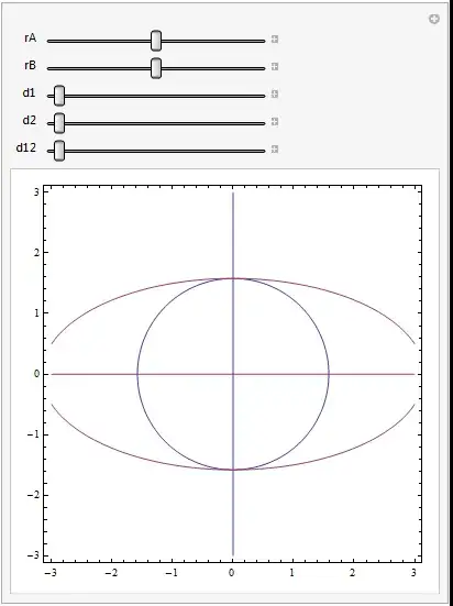
Second attempt, a graphical one:
Manipulate[
 ContourPlot[equations, {x, -10, 10}, {y, -10, 10},
  PlotPoints -> ControlActive[10, 50],
  MaxRecursion -> ControlActive[1, 10]], {r, -2, 2}, {r', -2, 2}, {d1,
   0, 10}, {d2, 0, 10}, {d12, 0, 10}]
Such approach would be preferential as one would then really be able to play with the parameters and learn all about the system and its solutions (e.g. how many of them etc). But I don't know if the contourplot is a good idea because I can't make any sense of the results yet, added to which it is a bit difficult to guess the right range of values for the variables and parameters.
- Can anyone come up with suggestions that can improve any of the two attempts?
result = Reduce[equations, {x, y}, Reals]`
– Daniel Lichtblau Apr 20 '15 at 15:31