I am putting all of my code in one block for easy copy and paste.
sys = {u (1 - u + a v), r v (1 - v + b u)};
sys1 = sys /. {a -> 2, b -> 3, r -> 1};
equilibria = Solve[sys1 == {0, 0}];
equilibria = equilibria[[{2, 3, 4}]];
sol[{u0_, v0_}] :=
  NDSolveValue[{{u'[t],
      v'[t]} == (sys1 /. {u -> u[t], v -> v[t]}), {u[0], v[0]} == {u0,
       v0},
    WhenEvent[Abs[u[t] - 1] > 1, "StopIntegration"],
    WhenEvent[Abs[v[t] - 1] > 1, "StopIntegration"]}, {u[t],
    v[t]}, {t, -4, 4},
   "ExtrapolationHandler" -> {Indeterminate &,
     "WarningMessage" -> False}];
initconds = {{0.1, 1.5}, {1.5, 0.1}, {0.1, 0.5}, {0.5, 0.1}};
toplot = Map[sol, initconds];
plt = ParametricPlot[toplot, {t, -4, 4}, PlotStyle -> Blue];
Show[vp, cp, plt,
 Graphics[{Red, PointSize[Large], Point[{u, v}] /. equilibria,
   Text[Style["(0,0) nodal source", Black, Background -> White], {0.1,
      0.1}],
   Text[Style["(1,0) saddle", Black, Background -> White], {1, 0.1}],
   Text[Style["(0,1) saddle", Black, Background -> White], {0.1,
     1.1}]}]]
The resulting figure follows.

I've only tested these concepts one time, on this one system. I am wondering what folks think. Will I get in trouble in general?
Grisha's Suggestion:
Clear["Global`*"];
sys = {u (1 - u + a v), r v (1 - v + b u)};
sys1 = sys /. {a -> 2, b -> 3, r -> 1};
vp = VectorPlot[sys1, {u, -0.1, 2}, {v, -0.1, 2},
   VectorScale -> {0.045, 0.9, None},
   VectorStyle -> {GrayLevel[0.8]},
   Axes -> True, AxesLabel -> {x, y}, AxesOrigin -> {0, 0}];
cp = ContourPlot[sys1, {u, -0.1, 2}, {v, -0.1, 2},
   ContourStyle -> {Orange, Green}];
equilibria = Solve[sys1 == {0, 0}];
equilibria = equilibria[[{2, 3, 4}]];
initconds = {{0.1, 1.5}, {1.5, 0.1}, {0.1, 0.5}, {0.5, 0.1}};
sp = StreamPlot[sys1, {u, -0.5, 2}, {v, -0.5, 2}, StreamScale -> None,
    StreamPoints -> initconds,
   StreamStyle -> {Blue, "Line"}];
Show[vp, cp, sp,
 Graphics[{Red, PointSize[Large], Point[{u, v}] /. equilibria,
   Text[Style["(0,0) nodal source", Black, Background -> White], {0.1,
      0.1}],
   Text[Style["(1,0) saddle", Black, Background -> White], {1, 0.1}],
   Text[Style["(0,1) saddle", Black, Background -> White], {0.1,
     1.1}]}]]

One can see that Grisha's suggestion worked nicely here.
Case where ab<1
Clear["Global`*"];
sys = {u (1 - u + a v), r v (1 - v + b u)};
sys2 = sys /. {a -> 1/3, b -> 1/4, r -> 1};
vp2 = VectorPlot[sys2, {u, -0.1, 2}, {v, -0.1, 2},
VectorScale -> {0.045, 0.9, None},
VectorStyle -> {GrayLevel[0.8]},
Axes -> True, AxesLabel -> {x, y}, AxesOrigin -> {0, 0}];
cp2 = ContourPlot[sys2, {u, -0.1, 2}, {v, -0.1, 2},
ContourStyle -> {Orange, Green}];
equilibria = Solve[sys2 == {0, 0}];
initconds2 = {{0.1, 1.5}, {1.5, 0.1}, {0.1, 0.5}, {0.5, 0.1}, {0.7,
2}, {2, 2}, {2, 0.7}};
sp2 = StreamPlot[sys2, {u, -0.1, 2}, {v, -0.1, 2},
StreamScale -> None, StreamPoints -> initconds2,
StreamStyle -> {Blue, "Line"}];
Show[vp2, cp2, sp2,
Graphics[{Red, PointSize[Large], Point[{u, v}] /. equilibria,
Text[Style["(0,0) nodal source", Black, Background -> White], {0.1,
0.1}],
Text[Style["(1,0) saddle", Black, Background -> White], {1, 0.1}],
Text[Style["(0,1) saddle", Black, Background -> White], {0.1, 1.1}],
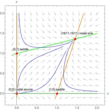
Text[Style["(16/11,15/11) nodal sink", Black,
Background -> White], {1.5, 1.5}]}]]
Produces the following image.
Notice that it failed to use three initial conditions. Changing the initial condition {0.7, 2} to {0.7,1.9} fixes the problem.
Clear["Global`*"];
sys = {u (1 - u + a v), r v (1 - v + b u)};
sys2 = sys /. {a -> 1/3, b -> 1/4, r -> 1};
vp2 = VectorPlot[sys2, {u, -0.1, 2}, {v, -0.1, 2},
   VectorScale -> {0.045, 0.9, None},
   VectorStyle -> {GrayLevel[0.8]},
   Axes -> True, AxesLabel -> {x, y}, AxesOrigin -> {0, 0}];
cp2 = ContourPlot[sys2, {u, -0.1, 2}, {v, -0.1, 2},
   ContourStyle -> {Orange, Green}];
equilibria = Solve[sys2 == {0, 0}];
initconds2 = {{0.1, 1.5}, {1.5, 0.1}, {0.1, 0.5}, {0.5, 0.1}, {0.7,
    1.9}, {2, 2}, {2, 0.7}};
sp2 = StreamPlot[sys2, {u, -0.1, 2}, {v, -0.1, 2},
   StreamScale -> None, StreamPoints -> initconds2,
   StreamStyle -> {Blue, "Line"}];
Show[vp2, cp2, sp2,
 Graphics[{Red, PointSize[Large], Point[{u, v}] /. equilibria,
   Text[Style["(0,0) nodal source", Black, Background -> White], {0.1,
      0.1}],
   Text[Style["(1,0) saddle", Black, Background -> White], {1, 0.1}],
   Text[Style["(0,1) saddle", Black, Background -> White], {0.1, 1.1}],
   Text[Style["(16/11,15/11) nodal sink", Black,
     Background -> White], {1.5, 1.5}]}]]
Giving the following image.

Not bad, not bad at all. Curious why I had to make the initial condition point change I made.
However, note that now all the stream plots don't push very close to the nodal sink. Is there a way you can force them to move a bit closer?
My Technique Again My technique seemed to work again.
Clear["Global`*"];
sys = {u (1 - u + a v), r v (1 - v + b u)};
sys2 = sys /. {a -> 1/3, b -> 1/4, r -> 1};
vp2 = VectorPlot[sys2, {u, -0.1, 2}, {v, -0.1, 2},
   VectorScale -> {0.045, 0.9, None},
   VectorStyle -> {GrayLevel[0.8]},
   Axes -> True, AxesLabel -> {x, y}, AxesOrigin -> {0, 0}];
cp2 = ContourPlot[sys2, {u, -0.1, 2}, {v, -0.1, 2},
   ContourStyle -> {Orange, Green}];
equilibria = Solve[sys2 == {0, 0}];
sol[{u0_, v0_}] :=
  NDSolveValue[{{u'[t],
      v'[t]} == (sys2 /. {u -> u[t], v -> v[t]}), {u[0], v[0]} == {u0,
       v0},
    WhenEvent[Abs[u[t] - 1] > 1, "StopIntegration"],
    WhenEvent[Abs[v[t] - 1] > 1, "StopIntegration"]}, {u[t],
    v[t]}, {t, -4, 4},
   "ExtrapolationHandler" -> {Indeterminate &,
     "WarningMessage" -> False}];
initconds2 = {{0.1, 1.5}, {1.5, 0.1}, {0.1, 0.5}, {0.5, 0.1}, {0.7,
    1.9}, {2, 2}, {2, 0.7}};
toplot2 = Map[sol, initconds2];
plt2 = ParametricPlot[toplot2, {t, -4, 4}, PlotStyle -> Blue];
Show[vp2, cp2, plt2,
 Graphics[{Red, PointSize[Large], Point[{u, v}] /. equilibria,
   Text[Style["(0,0) nodal source", Black, Background -> White], {0.1,
      0.1}],
   Text[Style["(1,0) saddle", Black, Background -> White], {1, 0.1}],
   Text[Style["(0,1) saddle", Black, Background -> White], {0.1, 1.1}],
   Text[Style["(16/11,15/11) nodal sink", Black,
     Background -> White], {1.5, 1.5}]}]]
Producing this image:

However, this time I got a couple warning messages:

I'd love to hear suggestions from folks.
{2,2}and{2,0.7}start on the boundary of theWhenEventconditions; in such a case, theWhenEventis ignored andNDSolvetries to integrate to infinity.WhenEventonly detects crossing a boundary. If you change each2to1.99, no messages are generated. (3) I don't quite understand the purpose of theContourPlot. – Michael E2 Apr 22 '15 at 21:48