For a physics application I am considering the radial Bogoliubov-de Gennes equations in two dimensions. In dimensionless form they read as follows $$ \begin{cases} \bigg[\frac{1/4-m^2}{r^2}+2(E-1)\bigg] u_m(r)-2v_m(r)+u_m''(r)=0 \newline \bigg[\frac{1/4-m^2}{r^2}-2(E+1)\bigg] v_m(r)-2u_m(r)+v_m''(r)=0, \end{cases} $$ where $m = 0,1,2$ and $E$ is the energy, a continuous parameter. In fact, one can show that $$ \begin{cases} u_m(r) = -\frac{2\sqrt{r}J_m(kr)}{2+k^2-2E} \newline v_m(r) = \sqrt{r}J_m(kr) \end{cases} $$ is a solution for $k = \sqrt{2(\sqrt{1+E^2}-1)}$ by explicitly substituting it in the equations.
At some point I want to multiply the off-diagonal terms in the system of equations by a function of the radius $r$. This will not be exactly solvable. Hence, I would like to understand how to numerically solve these equations in Mathematica before I make the equations more difficult.
The code I have up to now, is the following:
BdGplot[E1_, Bc1_, m1_] :=
Module[{E = E1, Bc = Bc1, m = m1}, {btc = 50,
k = Sqrt[2]*Sqrt[-1 + Sqrt[1 + E^2]],
uw = -(2 /(2 + k^2 - 2E)),
ub[r_] := (2/Pi)^(1/2)*uw*Cos[k*r - m*Pi/2 - Pi/4],
vb[r_] := (2/Pi)^(1/2)*Cos[k*r - m*Pi/2 - Pi/4],
s = NDSolve[{((1/4 - m^2)/r^2 + 2 (-1 + E)) u[r] -
2 v[r] + u''[r] == 0, -2 u[r] + ((1/4 - m^2)/r^2 - 2(1 + E)) v[r] + v''[r] == 0, u[Bc] == ub[Bc], u'[Bc] == ub'[Bc], v[Bc] == vb[Bc], v'[Bc] == vb'[Bc]}, {u,v}, {r, 1/1000, btc}]};
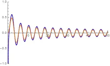
Plot[Evaluate[{u[r]/(uw*Sqrt[r]), v[r]/Sqrt[r],
BesselJ[m, k*r]} /. s], {r, 0.001, btc},
PlotRange -> {{0, btc}, {-2, 2}}, PlotStyle -> {Red, Blue, Orange}]
]
The idea is to give boundary conditions at large distance $r$ which are the asymptotic values of the m-th Bessel functions (in the more difficult case, the boundary conditions will be similar). Subsequently I let Mathematica numerically integrate the equations to a small radius $r=0.001$, such that it does not run into trouble at $r=0$.
However, plotting with a command like plotAlpha1 = Manipulate[BdGplot[1.5, Bc, 0], {Bc, 1, 50, 1/10}], one sees that the numerical solutions only match to the exact solution in a certain region. At some point the solutions diverge heavily. Does anybody have any idea how I can resolve this issue?

WorkingPrecision -> 50which will improve the situation a lot. You will have to take care that all constants will be given as exact numbers, but that would only mean to change1.5to3/2for the value in theManipulate... – Albert Retey Jun 05 '15 at 09:37WorkingPrecision->30should be good enough, and I forgot to mention that this is of course to be used as an option toNDSolve... – Albert Retey Jun 05 '15 at 09:521.5to3/2is necessary, orWorkingPrecision -> 32won't work at all! I used to think that though the warningNDSolve::precwwill be generated, as long as a higherWorkingPrecisionis set, approximate numbers in the differential equation won't influence the result. (Actually I never saw this principle failed before!) – xzczd Jun 05 '15 at 13:36