How to combine ParametricPlot and RegionPlot?

Question

I have two implicitly defined equations. I plot the implicit curve using parametric plot.

k3 = 0.4;
n = 4;
k1 = 3;

k2 = (k3*((n - 1)*(s1/k1)^n - 1))/(1 + (s1/k1)^n)^2;
v1 = k2*s1 + (k3*s1)/(1 + (s1/k1)^n);

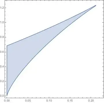
ParametricPlot[{k2, v1}, {s1, 0.0, 50}, 
PlotRange -> {{0, 0.3}, {0, 1.5}}, AspectRatio -> 0.5, 
PlotStyle -> Black]

enter image description here

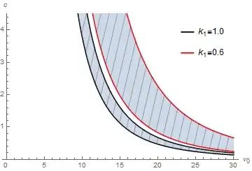
Now I want to color and hatch the area inside. In another project I used RegionPlot for this (see an example below), but how can I use RegionPlot (or some other technic perhaps) for this example with implicit equations?

enter image description here

Strongly related: "Generating hatched filling." – Alexey Popkov May 05 '15 at 17:18 — Alexey Popkov, May 05 '15 at 17:18

score 11 · Answer 1 · answered May 05 '15 at 17:37

11

Probably this match your plot:

ParametricPlot[{r {r k2, v1}}, {s1, 0.0, 50}, {r, 0, 1}, 
 PlotRange -> {{0, 0.3}, {0, 1.5}}, AspectRatio -> 0.5, 
 BoundaryStyle -> Directive[Black, Thick], Mesh -> 100, 
 MeshFunctions -> (50 #1 - #2 &)]

enter image description here

answered May 05 '15 at 17:37

Basheer Algohi

19,917
1
31
78

Nice! I have tried almost all the wrong ways to get the third argument of ParametricPlot working:) ( +1) – kglr May 05 '15 at 17:54
2

some more explanations on the parameterization would be of great help, though that might be more related to math rather than Mathematica:) But definitely an elegant answer! – sunt05 May 05 '15 at 17:57
Great! Thank you! – Alex Ivanov May 05 '15 at 18:02
@kguler, Well I am now very prouder. +1 from you is a big thing because it is not an easy task to impress you:) – Basheer Algohi May 05 '15 at 18:03
@Algohi, see vote counts:) By the way, this answer is not an exception by any means -- I learned a lot from your answers; I don't remember one that I wasn't impressed with or did not upvote. – kglr May 05 '15 at 18:13
@kguler I may not express my feeling toward you correctly. I meant you are great. sorry if my words are not correct. – Basheer Algohi May 05 '15 at 18:16

score 10 · Accepted Answer · edited Apr 13 '17 at 12:55

10

To fill with a solid color, you can post-process the Line primitive into a Polygon

ParametricPlot[{k2, v1}, {s1, 0.0, 50}, 
 PlotRange -> {{0, 0.3}, {0, 1.5}}, AspectRatio -> 0.5, 
 PlotStyle -> Black] /. Line[x_] :> {Blue, Polygon[x]}

Mathematica graphics

Update: Using the approach in this answer mentioned in Alexey's comment:

poly = Cases[pp, Line[x_] :> Polygon[x], {0, Infinity}][[1]]; 
Quiet[region = Region`RegionProperty[poly, {x, y}, "FastDescription"][[1, 2]]];

RegionPlot[region, {x, 0, .3}, {y, 0, 1.5}, Mesh -> 50, 
 MeshFunctions -> {#1 - #2 &}, MeshStyle -> White, 
 PlotStyle -> Directive[{Thick, Blue}], PlotPoints -> 100]

Mathematica graphics

edited Apr 13 '17 at 12:55

Community

1

answered May 05 '15 at 16:54

kglr

394,356
18
477
896

Wow, so smart! but I'm still wondering if there is a way to convert this to be suitable for RegionPlot. – sunt05 May 05 '15 at 16:58
@sunt05, please see the update using the same trick in the linked answer. – kglr May 05 '15 at 17:51

score 1 · Answer 3 · answered May 05 '15 at 18:07

If you absolutely, positively insist on using RegionPlot, then it's still possible to do with the curve you mentioned. This is because it's actually possible for your curve to be written as $v_1(k_2)$, albeit in a pretty ugly form. Start by inverting your relation between $s_1$ and $k_2$:

s1solns = Solve[(k3*((n - 1)*(s1/k1)^n - 1))/(1 + (s1/k1)^n)^2 == k2, s1];

Ugly solutions for s1(k2)

Once you've got that, you can replace $s_1$ with these functions of $k_2$ in your expression for $v_1$. This gives you two functions for $v_1(k_2)$; the desired region is bounded above by the first function, and below by the second function. Note that $k_2$ has a maximum value for which these functions are real, which I call $k_{2\text{max}}$ in the code below.

params = {k3 -> 0.4, n -> 4, k1 -> 3}; 
v1curves = (k2*s1 + (k3*s1)/(1 + (s1/k1)^n) /. s1solns) /. params;
k2max = k2 /. First[Solve[((k3^2 - 4 k2 k3 n - 2 k3^2 n + k3^2 n^2) /. params) == 0, k2]];
RegionPlot[
 v1 <= v1curves[[1]] && v1 >= v1curves[[2]] && k2 >= 0, 
 {k2, 0, k2max}, {v1, 0, Evaluate[v1curves[[1]] /. k2 -> k2max]}, 
 MaxRecursion -> 6]

enter image description here

This method is, to be honest, a kludgey hack; the above answers are much better, and will generalize much more readily. But it was still fun to try to do this with one hand tied behind my back. :-)

How to combine ParametricPlot and RegionPlot?

3 Answers3