The envelope of a set of translated and rotated ellipses

Question

I achieve a dynamic graphics by using Manipulate as follows:

Manipulate[
 ParametricPlot[
  RotationMatrix[β].{a + c Cos[Θ], b + d Sin[Θ]}, {Θ, 0, 2 π}, 
  PlotRange -> {{-15, 15}, {-15, 15}}],
 {{a, 1}, 0, 5, 1, Appearance -> "Labeled"},
 {b, 0, 6, 1}, {c, 1, 5, 1}, 
 {d, 2, 6, 1}, {β, 0, π, 1}]

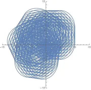
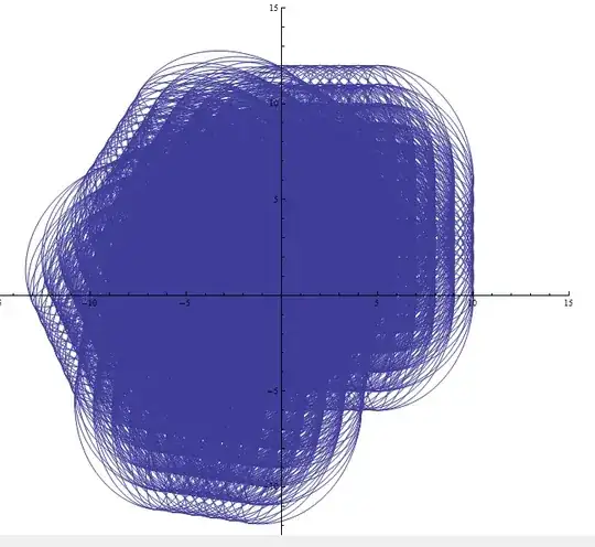
To see the dynamic region, I do the following operation:

Table[
 ParametricPlot[
  RotationMatrix[β].{a + c Cos[Θ], b + d Sin[Θ]}, {Θ, 0, 2 π}, 
  PlotRange -> {{-15, 15}, {-15, 15}}],
 {a, 0, 5, 1},
 {b, 0, 6, 1}, {c, 1, 5, 1}, 
 {d, 2, 6, 1}, {β, 0, π, 1}]// Flatten // Show

In addition, I noticed that

ParametricPlot[
 r^2 { Sqrt[t] Cos[t], Sin[t]}, {t, 0, 3 π/2}, {r, 1, 2}]

can give a region of a dynamic graphic. However, it cannot work when the parameters exceed 2

Question

Is it possible to achieve the envelope line of a set of dynamic graphs ? It is my first time to think out this question and I have no idea.

You have an envelope of parametrically-defined curves; as noted here or here (en Français, sorry), you can derive the envelope's parametric equations by eliminating the free parameter from the parametric equations and the determinant of its partial derivatives. — J. M.'s missing motivation, May 16 '15 at 06:41
@Guesswhoitis. The problem, as I see it, is that the free parameters are discrete. If they were continuous, the bounding curve would be simply a circle. — bbgodfrey, May 16 '15 at 14:37
@bbgodfrey, true; that makes computing an explicit representation of the envelope harder. — J. M.'s missing motivation, May 16 '15 at 14:43

bbgodfrey · Accepted Answer · 2015-05-16T15:23:17.943

This problem can be simplified substantially by noting that only the largest ellipses contribute to the boundary of the second figure in the question. So, for instance,

Table[ParametricPlot[RotationMatrix[β].{a + 5 Cos[Θ], b + 6 Sin[Θ]}, {Θ, 0, 2 Pi}, 
  PlotRange -> {{-15, 15}, {-15, 15}}], {a, 0, 5, 1}, {b, 1, 6, 1}, {β, 0, Pi, 1}]
  // Flatten // Show

enter image description here

Furthermore, this plot is seen to be the composite of four objects,

Table[ParametricPlot[{a + 5 Cos[Θ], b + 6 Sin[Θ]}, {Θ, 0, 2 Pi}, 
  PlotRange -> {{-15, 15}, {-15, 15}}], {a, -2.5, 2.5, 1}, {b, -2.5, 2.5, 1}]
  // Flatten // Show

enter image description here

each one displaced by the average values of a and b, {2.5, 3.0} in this case, and rotated by the four values of β.

Continuation

The region corresponding to the previous plot is approximately (exactly in the limit of continuous a and b) is

r = RegionUnion[Flatten[{
    Table[Ellipsoid[{a, b}, {5, 6}], {a, -2.5, 2.5, 5}, {b, -2.5, 2.5, 5}], 
    Rectangle[{-2.5, -8.5}, {2.5, 8.5}], Rectangle[{-7.5, -2.5}, {7.5, 2.5}]}]];
RegionPlot[r, PlotRange -> {{-15, 15}, {-15, 15}}]

enter image description here

This region then is translated by {2.5, 3.0} and rotated by β.

t = TransformedRegion[r, TranslationTransform[{2.5, 3}]];
s = RegionUnion[Table[TransformedRegion[t, RotationTransform[β]], {β, 0, Pi, 1}]];

The boundary of s is the desired surface.

u = RegionBoundary[s];
RegionPlot[u, PlotRange -> {{-15, 15}, {-15, 15}}]
DeleteCases[%, Line[{_, _}] | Point[__], Infinity]

enter image description here

The last line of code eliminates most spurious points and point-like lines that mysteriously (to me) otherwise appear.

Warning: Trying to plot s itself promptly devoured all the memory on my PC.

This is very elegant. I had been thinking about this problem since the question came out, but I had gotten nowhere. Thanks for putting me out of my misery! (+1) — MarcoB, May 16 '15 at 22:11

score 6 · Answer 2 · answered May 16 '15 at 22:41

6

The general idea is the same as bbgodfrey's so most credits for him, the approach is slightly different, perhaps more automatic.

We start by converting OP's parametric expression to cartesian:

eq = #.# &@{Cos[Θ], Sin[Θ]} /. Solve[
     Thread[{x, y} == RotationMatrix[β].{a + c Cos[Θ], b + d Sin[Θ]}],
     {Cos[Θ], Sin[Θ]}
     ][[1]] // Simplify

(regions = Table[
      ImplicitRegion[eq <= 1, {x, y}],
      {a, 0, 5, 1}, {b, 0, 6, 1}, {c, 5, 5, 1}, {d, 6, 6, 1}, {β, 0, π, 1}
 ] // Flatten // N);
 (*only the biggest c and d as noticed by bbdogfrey*)

RegionUnion[regions] // DiscretizeRegion[#, AccuracyGoal -> 3] & // 
   RegionBoundary // AbsoluteTiming

enter image description here

answered May 16 '15 at 22:41

Kuba

136,707
13
279
740

Kuba, elegant solution. Well done. Do you understand why using DiscretizeRegion[#]] & // RegionBoundary decreases running time by orders of magnitude, compared to RegionBoundary // RegionPlot? – bbgodfrey May 17 '15 at 00:42
Shutao Tang, although I cannot speak for Kuba, I would note that DiscretizeRegion is new to Mathematica 10. – bbgodfrey May 17 '15 at 00:44
@bbgodfrey I don't know, I'm not so much experienced in Regions. :/ – Kuba May 17 '15 at 06:45
@ShutaoTang Yes, this is V10 solution. You could try to mimic this. Plot filled ellipses, extract polygons, find here a function to merge polygons (it is somewhere, I don't know where). Fold this operation on a list of ellipses and you have a solution. Probably, haven;t tested it and don't have time :/ – Kuba May 17 '15 at 06:47
@Kuba, Thanks very much sincerely:-) – xyz May 17 '15 at 06:51

score 4 · Answer 3 · edited Apr 13 '17 at 12:55

Here is an approach came from this answer and bbgodfrey's answer. In addition, it is very fast.

s = 
  DiscretizeGraphics@
    Graphics[Polygon /@ 
      Table[Table[{a + 5 Cos[theta], b + 6 Sin[theta]}, 
      {theta, 0, 2 Pi, 0.02 Pi}], {a, -2.5, 2.5, 1}, {b, -2.5, 2.5, 1}]]

enter image description here

t = TransformedRegion[s, TranslationTransform[{2.5, 3}]];
RegionBoundary@
  RegionUnion[
   Table[TransformedRegion[t, RotationTransform[beta]], {beta, 0, Pi, 1}]]

enter image description here

The envelope of a set of translated and rotated ellipses

Question

3 Answers3