A bug in Integrate

Question

Integrate[(1 + 16 Tan[2 x - y]^2)/(1 + 4 Tan[2 x - y]^2), {x, 0, 2 π}]

Mathematica (wrong) output is (tested under versions 8 and 10.0, took ~ 1 minute of CPU time)

10 π

The correct value of this integral is 6 π (not 10 π).

Integrate[(1 + 16 Tan[2 x - 2]^2)/(1 + 4 Tan[2 x - 2]^2), {x, 0, 2 π}]
(* 6 π *)
Integrate[(1 + 16 Tan[2 x - 4]^2)/(1 + 4 Tan[2 x - 4]^2), {x, 0, 2 π}]
(* 6 π *)

Version 8 and 10.0.0.0 Version 7.0.1.0

Answer 1

I've got a theory....

Let's try to get the antiderivative:

Integrate[(1 + 16*Tan[2*x - y]^2)/(1 + 4*Tan[2*x - y]^2), x,
 Assumptions -> y \[Element] Reals]

(*returns 5 x - (5 y)/2 - ArcTan[2 Tan[2 x - y]] *)

Seems legit. You can test with D[5 x - (5 y)/2 - ArcTan[2 Tan[2 x - y]], x] and plot or rearrange. This antiderivative is technically correct, but there is a latent +k Pi missing where k is an integer.

Using the antiderivative and the fundamental theorem of calculus you can evaluate at 2 Pi and 0 and subtract the first from last giving 10 Pi. Yet if you use NIntegrate (for some random numerical y), it converges to 6 Pi as expected... so a mystery 4 Pi has been added that vanished when the singularities in both the numerator and denominator of the integrand became removable as a fraction.

I think what's happening is Mathematica is not accommodating ArcTan and Tan's branch cuts at these singularities which will result in an extra +k Pi being added on, in this case it's an extra 4 Pi on top of the true answer. Those branch cut singularities in the top and bottom of the fraction are supposed to disappear (become removable) if we're just dealing with real numbers - yet Mathematica fails to realize this. Why 4 Pi? Well probably because if you plot the denominator or numerator you'll always see exactly 4 singularities for any choice of y. For instance try setting y to 5 and doing:

Show[Plot[(1 + 16*Tan[2*x - y]^2) /. y -> 5, {x, 0, 2 Pi}], 
     Plot[(1 + 4*Tan[2*x - y]^2) /. y -> 5, {x, 0, 2 Pi}]]

If we now force y and x to only use the real part we get the answer without the mystery +4 Pi

Integrate[(1 + 16*Tan[2*Re[x] - Re[y]]^2)/(1 + 4*Tan[2*Re[x] -
 Re[y]]^2), {x, 0, 2 Pi}] 

(*Answer 6 Pi *)

It's just a theory of mine; I've only recently been studying complex analysis so I may not be right... I definitely think it's a bug now.

EXTRA: to show that my D[...antiderivative...,x] and the integrand are equivalent you can do:

TrigReduce[5 - (4 Sec[2 x - y]^2)/(1 + 4 Tan[2 x - y]^2)] == 
TrigReduce@FullSimplify[(1 + 16 Tan[2 x - y]^2)/(1 + 4 Tan[2 x - y]^2)]

Answer 2

[Edit notice: I'll put the gist up front.]

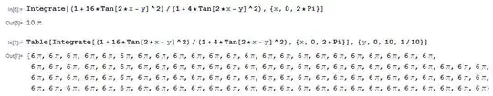
10 π is not wrong

With proper assumptions given, the integral evaluates as desired by the OP, to 6 π. Without them, it gives one of the correct values of the integral, 10 π, the one that in some sense is more likely, but without the correct conditions attached. (One may well argue that is a bug. However, Mathematica's exact solvers usually give only generically correct solutions. And beyond that, Integrate is a little looser than the others, and that is, I suspect, so that it can reach answers within a reasonable amount of time, when they can be reached at all. No doubt everyone wishes for more accurate and reliable algorithms.)

By default Mathematica's functions treat variables as complex numbers. These include functions called by Integrate. Clearly in the OP's call

Integrate[(1 + 16 Tan[2 x - y]^2)/(1 + 4 Tan[2 x - y]^2), {x, 0, 2 π}]

the variable y should be treated as complex. What's less clear is whether in the line integral from x == 0 to x = 2 Pi, the variable x should be considered real. In fact, it need not be. Sometimes it can help to explicitly specify that x is real or even 0 < x < 2 Pi.

Integrate[(1 + 16 Tan[2 x - y]^2)/(1 + 4 Tan[2 x - y]^2),
 {x, 0, 2 π}, Assumptions -> -(π/2) <= y <= π/2 && 0 < x < 2 Pi]
(*  6 π  *)

In fact this result is valid only when Abs[Im[y]] < Log[3]/2. When Abs[Im[y]] > Log[3]/2, the integral is 10 π. (So on the basis of the length of the intervals, for most values of y the integral is 10 π.)

Interestingly this is one of those cases where Assuming and Assumptions give different results:

Assuming[-(π/2) <= y <= π/2 && 0 < x < 2 Pi,
 Integrate[(1 + 16 Tan[2 x - y]^2)/(1 + 4 Tan[2 x - y]^2), {x, 0, 2 π}]]
(*  10 π  *)

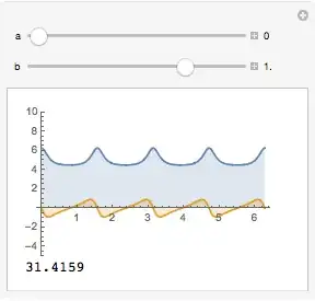
One can see the difference in the graph of the integrand. Just by estimating the the average height of the graph, one can see the results 6 π, 10 π are probably correct in their respective cases.

Manipulate[
 Column[{
   Plot[Evaluate@
     Through[{Re, Im}[(1 + 16*Tan[2*x - y]^2)/(1 + 4*Tan[2*x - y]^2) /. y -> a + b I]],
    {x, 0, 2 Pi}, AxesOrigin -> {0, 0}, 
    PlotRange -> {-5, 10}, Filling -> Axis, ImageSize -> 225],
   Chop[N@
     NIntegrate[(1 + 16 Tan[2 x - y]^2)/(1 + 4 Tan[2 x - y]^2) /. y -> SetPrecision[a + b I, Infinity],
      {x, 0, 2 π}, 
      PrecisionGoal -> 10, WorkingPrecision -> 50, 
      MaxRecursion -> 16], 1*^-15]
   }],
 {a, 0, 3, Appearance -> "Labeled", ImageSize -> 200},
 {b, -2, 2, Appearance -> "Labeled", ImageSize -> 200}]

Checking with NIntegrate

I get 10 Pi with y = I:

Block[{y = I},
 N@NIntegrate[(1 + 16 Tan[2 x - y]^2)/(1 + 4 Tan[2 x - y]^2),
    {x, 0, 2 π}, WorkingPrecision -> 25]]
% == 10 Pi
(*
  31.4159 + 0. I
  True
*)

Other times, I get 8 Pi:

Block[{y = 1 + I},
 N@NIntegrate[(1 + 16 Tan[2 x - y]^2)/(1 + 4 Tan[2 x - y]^2),
    {x, 0, I, 2 π}, WorkingPrecision -> 25]]
% == 8 Pi
(*
  25.1327 + 0. I
  True
*)

And sometimes I can even get 9 Pi:

Block[{y = 10},
 N@NIntegrate[(1 + 16 Tan[2 x - y]^2)/(1 + 4 Tan[2 x - y]^2),
    {x, 0, I, 2 π}, WorkingPrecision -> 25]]
% == 9 Pi
(*
  28.2743 + 0. I
  True
*)

However, this is interesting:

Integrate[(1 + 16 Tan[2 x - y]^2)/(1 + 4 Tan[2 x - y]^2),
  {x, 0, y, 2 π}, Assumptions -> y ∈ Reals]
(*  ConditionalExpression[(23 π)/3, y == π/2]  *)

I think this is certainly wrong. NIntegrate gives 6 Pi for y = π/2.

Answer 3

Oddly, if you follow the hints given in the ConditionalExpressions you can get pointed to the right answer although constrained to an overly restrictive region.

$Version

"10.1.0 for Mac OS X x86 (64-bit) (March 24, 2015)"

expr = (1 + 16 Tan[2 x - y]^2)/(1 + 4 Tan[2 x - y]^2);

Integrate[expr, {x, 0, 2 Pi}]

ConditionalExpression[9*Pi, -(Pi/2) <= y <= (7*Pi)/2]

The wrong answer; however, using the stated conditions

Assuming[{-Pi/2 <= y <= 7 Pi/2},
 Integrate[expr, {x, 0, 2 Pi}]]

ConditionalExpression[6*Pi, 2*y < Pi]

Applying the refined condition

Assuming[{-Pi/2 <= y <= Pi/2},
 Integrate[expr, {x, 0, 2 \[Pi]}]]

6*Pi

Integrate[expr /. y -> 100 Pi, {x, 0, 2 Pi}]

6*Pi

NIntegrate[expr /. y -> 100 Pi, {x, 0, 2 Pi}]

18.8496

Answer 4

Integrate and NIntegrate agree on this matter:

Table[Integrate[(1+16 Tan[2 x-y]^2)/(1+4 Tan[2 x-y]^2),{x,0,2Pi}],{y,0,10,2}]
(*==> {6π,6π,6π,6π,6π,6π}*)

Table[NIntegrate[(1+16 Tan[2 x-y]^2)/(1+4 Tan[2 x-y]^2),{x,0,2Pi}],{y,0,10,2}]
(*==> {18.8496,18.8496,18.8496,18.8496,18.8496,18.8496}*)

N[6Pi]
(*==> 18.8496*)