Can A Plot Be Overlayed With A Map?

Question

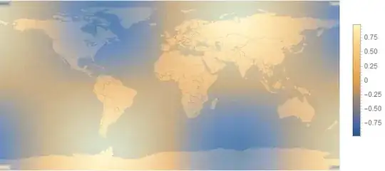
Some brief, only slightly important background. I am doing a research project using the data from NASA's GRACE mission. I wrote a short Perl script to take two data files and find the change in groundwater between the two dates. This gave me a set of 64,800 3D coordinates (One for every degree latitude and longitude on the Earth's surface). Using Mathematica, I created a ListDensityPlot to visualize the changes in groundwater. As you can see from the code below, the way I deal with clipping is pretty clumsy and doesn't look very good on the map. Otherwise, I am pretty happy with this plot. It pretty well shows everything I want it to. Most of the code courtesy of @Mr.Wizard.

den = ListDensityPlot[jpl200313,ColorFunction ->(ColorData["ThermometerColors"][1 - #] &),
    ClippingStyle -> {RGBColor[0.5, 0.02, 0.03],RGBColor[0, 0.01, 0.56]},
    PlotLegends ->BarLegend[Automatic,LegendMarkerSize -> 180,LegendFunction -> "Frame",
    LegendMargins -> 5,LegendLabel -> "Water Level Change (cm)"],PlotRange -> {-20, 20}];
prim = First@Cases[den, Graphics[a_, ___] :> a, {0, -1}, 1];
geo = GeoGraphics[{Opacity[0.6], prim},GeoBackground -> GeoStyling["StreetMapNoLabels"], 
   ImageSize -> 1000];
geo~Legended~den[[2]]

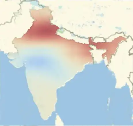
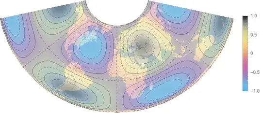
The final piece that I would like to figure out is how to narrow down to specific countries while keeping the legend. Eventually I will build a table or possibly an animate function of several maps of the same country with time being the manipulatable variable. These pictures are from code courtesy of @FJRA.

southamerica =ListDensityPlot[jpl200313, AspectRatio -> 1/2, Frame->None, 
   PlotRangePadding -> 0, PlotRange -> {-20, 20},ColorFunction ->
    (ColorData["ThermometerColors"][1 - #] &)];
img1 = Rasterize[southamerica, "Image", RasterSize -> 360];
img2 = SetAlphaChannel[img1, .8];
geoplot = GeoGraphics[{GeoStyling[{"GeoImage", img2},GeoRange -> {{-90, 90}, {-180, 180}}],
    Polygon[EntityClass["Country", "SouthAmerica"]]},GeoBackground ->
    GeoStyling["StreetMapNoLabels"],GeoZoomLevel -> 3,GeoProjection -> "Equirectangular"]

The code for the picture of India is identical except for the name and the Entity function.

Anyway, my big question at this point is whether or not the functionality of looking at individual countries can be combined with the readability of the first plot where I can add legends, titles labels etc. Thanks again!

Answer 1

Please see the Utility function section for a concise summary.

An arbitrary density plot for the example:

den = DensityPlot[Sin[x] Sin[y], {x, -180, 180}, {y, -90, 90}]

:

Extract the graphics primitives from the density plot:

prim = First @ Cases[den, Graphics[a_, ___] :> a, {0, -1}, 1];

Plot them directly with GeoGraphics while setting the desired GeoStyling for the GeoBackground:

GeoGraphics[
  {Opacity[0.8], prim},
  GeoBackground -> GeoStyling["ReliefMap"]
]

With GeoStyling["ContourMap"]:

ImageSize proves to be important; with "StreetMapNoLabels" an and and ImageSize of 512 or less no country borders are shown; 513 or greater and they are:

GeoGraphics[
  {Opacity[0.6], prim},
  GeoBackground -> GeoStyling["StreetMapNoLabels"], 
  ImageSize -> 600
]

---

Projections

To enable arbitrary projections we need to convert the plain coordinates in in the DensityPlot primitives to GeoPosition coordinates. prim as extracted above is a GraphicsComplex object which we can convert with:

prim2 = MapAt[GeoPosition @* Map[Reverse], prim, 1];

Now:

GeoGraphics[
  {Opacity[0.7], prim2},
  GeoBackground -> GeoStyling["StreetMapNoLabels"], 
  ImageSize -> 700,
  GeoProjection -> "Albers"
]

Legends

Including the legend from the original DensityPlot may be done like this:

den = DensityPlot[Sin[x] Sin[y], {x, -180, 180}, {y, -90, 90},
        PlotLegends -> Automatic];

prim = First @ Cases[den, Graphics[a_, ___] :> a, {0, -1}, 1];

geo = GeoGraphics[{Opacity[0.6], prim},
        GeoBackground -> GeoStyling["StreetMapNoLabels"], 
        ImageSize -> 600];

geo ~Legended~ den[[2]]

---

Utility function

The methods above may be combined into a single utility function.

toGeoGraphics[
  Shortest[opac : _?NumericQ : 0.6],
  opts : OptionsPattern[GeoGraphics]
][in_] :=
  With[{trans = If[MatchQ[OptionValue[GeoProjection], Automatic | "Equirectangular"], {},
     gc_GraphicsComplex :> MapAt[GeoPosition@*Map[Reverse], gc, 1]]},
    in /. Graphics[prim_, ___] :>
      GeoGraphics[{Opacity @ opac, prim /. trans}, opts, Options @ toGeoGraphics]
  ]

Define any default options that you want:

Options[toGeoGraphics] =
  {GeoBackground -> GeoStyling["StreetMapNoLabels"], 
   ImageSize -> 600};

Now use it like this:

DensityPlot[Sin[x] Sin[y], {x, -180, 180}, {y, -90, 90},
 PlotLegends -> Automatic] // 
   toGeoGraphics[GeoProjection -> "Mollweide"]

The first parameter of toGeoGraphics is the opacity; the remainder are any options you wish to pass to GeoGraphics, overriding defaults.

big = DensityPlot[Sin[x/38] Sin[y/25], {x, -180, 180}, {y, -90, 90}, 
  ColorFunction -> "CMYKColors", PlotPoints -> 100, MeshFunctions -> {#3 &, #3 &}, 
  Mesh -> {Range[-1, 1, 0.4], Range[-0.8, 0.8, 0.4]}, MeshStyle -> {Black, Dashed}, 
  PlotLegends -> Automatic];

big // toGeoGraphics[0.4, GeoProjection -> "Albers"]

Answer 2

I would prefer to use the "GeoImage" styling, because you can use other projections when using it.

Let's say you have data for the whole world in a matrix:

data = Table[
  Sin[x Degree] Sin[y Degree], {y, -90, 90}, {x, -180, 180}]

Then you use ListDensityPlot:

den1 = ListDensityPlot[data, AspectRatio -> 1/2, Frame -> None, 
  PlotRangePadding -> 0];

And convert it to an image, and add some transparency level:

img1 = Rasterize[den1, "Image", RasterSize -> 360];
img2 = SetAlphaChannel[img1, .5]

Then you can use GeoStyling with "GeoImage":

GeoGraphics[{GeoStyling[{"GeoImage", img2}, 
   GeoRange -> {{-90, 90}, {-180, 180}}], 
  FilledCurve[
   GeoPath[{{-90, -180}, {90, -180}, {90, 0}, {90, 180}, {-90, 
      180}, {-90, 0}}, "Rhumb"]]}, GeoRange -> "World", 
 GeoBackground -> GeoStyling["StreetMapNoLabels"], GeoZoomLevel -> 2]

As I said, the good thing is that you can project it (but be careful with the GeoPath, needs to be modified for some projections that are not defined in the poles):

GeoGraphics[{GeoStyling[{"GeoImage", img2}, 
   GeoRange -> {{-90, 90}, {-180, 180}}], 
  FilledCurve[
   GeoPath[{{-86, -180}, {86, -180}, {86, 0}, {86, 180}, {-86, 
      180}, {-86, 0}}, "Rhumb"]]}, GeoRange -> "World", 
 GeoBackground -> GeoStyling["StreetMapNoLabels"], GeoZoomLevel -> 2, 
 GeoProjection -> "Mercator"]

Or clip only an specific area:

GeoGraphics[{GeoStyling[{"GeoImage", img2}, 
   GeoRange -> {{-90, 90}, {-180, 180}}], 
  Polygon[EntityClass["Country", "SouthAmerica"]]}, 
 GeoBackground -> GeoStyling["StreetMapNoLabels"], GeoZoomLevel -> 3, 
 GeoProjection -> "LambertAzimuthal"]