Volumes of Revolution with detailed diagram

Question

All, In calculus I have to do images such as the following in helping explain technique to students. This one is by rotating $y=\sqrt x$ about the x-axis, an image copied from Stewart's Calculus textbook.

enter image description here

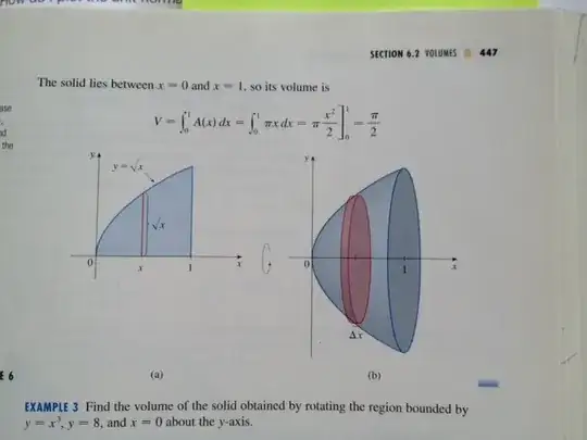
I am wondering if anyone has experience in doing this and has any links to share, some sample files, etc., which would give me an idea on how to best make the image on the right.

Thanks.

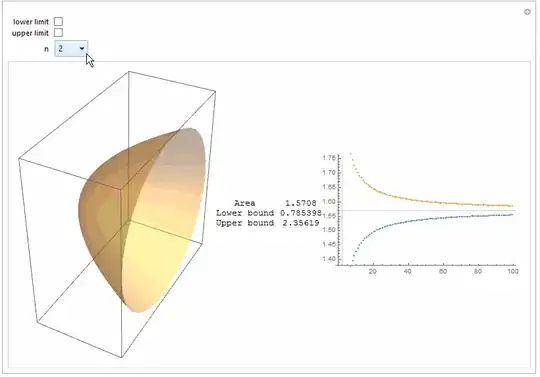
Close to what I need:

Consider:

Show[Plot[{-Sqrt[x], Sqrt[x]}, {x, 0, 1},
  PlotRange -> {{-0.25, 1.25}, {-1.5, 1.5}},
  PlotStyle -> Black,
  Filling -> True, FillingStyle -> Directive[LightBlue],
  AxesStyle -> Directive[Thin, Arrowheads[0.03]],
  Ticks -> {{1}, {-1, 1}},
  AxesLabel -> {"x", "y"},
  AspectRatio -> Automatic
  ],
 Graphics[{
   GrayLevel[0.7], EdgeForm[Black],
   Disk[{1, 0}, {.1, 1}],
   Pink,
   Rectangle[{0.47, -Sqrt[0.5]}, {0.53, Sqrt[0.5]}],
   Disk[{0.47, 0}, {.07, Sqrt[0.5]}],
   Disk[{0.53, 0}, {.07, Sqrt[0.5]}],
   Text[Style["\[CapitalDelta]x", Black], {0.5, -Sqrt[0.5]}, {0, 2}]
   }]
 ]

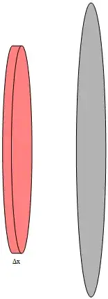
Which produces this image.

enter image description here

If I can come up with a way of joining (taking the union of) the first rectangle and first circle, so that the edge form only marks the exterior of the joined form, then I might have a solution. Any suggestions on how I might do that?

Final Update:

Thanks to @kguler's amazing answer, I learned an exceptional amount of material and possibilities. I made a few adjustments to his code. Here is my final example.

curve = Line@
   Table[{.53, 0} + {.07, Sqrt[0.5]} {Cos[t], Sin[t]}, {t, Pi/2, 
     3 Pi/2, Pi/20}];

poly = Polygon[
   Join[
    Table[{.53, 0} + {.07, Sqrt[0.5]} {Cos[t], Sin[t]}, {t, -Pi/2, 
      Pi/2, Pi/20}], 
    Table[{.47, 0} + {.07, Sqrt[0.5]} {Cos[t], Sin[t]}, {t, Pi/2, 
      3 Pi/2, Pi/20}]
    ]
   ];

g1 = Plot[{-Sqrt[x], Sqrt[x]}, {x, 0, 1}, 
   PlotRange -> {{-0.25, 1.25}, {-1.5, 1.5}}, PlotStyle -> Black, 
   Filling -> True, FillingStyle -> Directive[LightBlue], 
   AxesStyle -> Directive[Thin, Arrowheads[0.03]], 
   Ticks -> {{1}, {-1, 1}}, AxesLabel -> {"x", "y"}, 
   AspectRatio -> Automatic];

g2 = Graphics[{GrayLevel[0.7], EdgeForm[Black], Disk[{1, 0}, {.1, 1}],
     Pink, EdgeForm[Black], poly, Black, curve, 
    Text[Style["\[CapitalDelta]x", Black], {0.5, -Sqrt[0.5]}, {0, 
      2}]}];

Show[g1, g2, Graphics[{
   Blue, Line[{{0.5, 0}, {0.5, Sqrt[0.5]}}],
   Text[Style["\!\(\*SqrtBox[\(x\)]\)", Black, Bold], {0.5, 
     Sqrt[0.5]/2}, {-1.5, 0}],
   PointSize[Medium], Point[{0.5, 0}],
   Text[Style["x", Black, Bold], {0.5, 0}, {0, 1.5}]
   }]
 ]

And the resulting image:

enter image description here

Possibly related: Sketch-type graphics with transparency and dashed hidden lines. — Silvia, May 31 '15 at 19:16
I'd like to thank everyone for their answers. However, not quite what I am looking for. I have edited by original post with an attempt of what I'd like to use, but it sill is not quite adequate. — David, Jun 01 '15 at 05:03

kglr · Accepted Answer · 2015-06-01T06:56:50.170

Update:

a way of joining (taking the union of) the first rectangle and first circle, so that the edge form only marks the exterior of the joined form

p = 100; 
curve = Line@ Table[{.53, 0} + {.07, Sqrt[0.5]} {Sin[-2 Pi k /p], 
   Cos[-2 Pi k /p]}, {k, -1 + p/2}];
poly = Polygon[Join[t1 = Table[{.47, 0} + {.07, Sqrt[0.5]} {Sin[-2 Pi k /p], 
        Cos[-2 Pi k /p]}, {k, -1 + p/2}], 
   Reverse@Table[{.53, 0} + {.07, Sqrt[0.5]} {Sin[2 Pi k /p], Cos[2 Pi k /p]}, 
   {k, -1 + p/2}], {t1[[1]]}]]; 

g1 = Plot[{-Sqrt[x], Sqrt[x]}, {x, 0, 1}, 
  PlotRange -> {{-0.25, 1.25}, {-1.5, 1.5}}, PlotStyle -> Black, 
  Filling -> True, FillingStyle -> Directive[LightBlue], 
  AxesStyle -> Directive[Thin, Arrowheads[0.03]], 
  Ticks -> {{1}, {-1, 1}}, AxesLabel -> {"x", "y"}, AspectRatio -> Automatic];

g2 = Graphics[{GrayLevel[0.7], EdgeForm[Black], 
  Disk[{1, 0}, {.1, 1}], Pink, EdgeForm[Black], poly, Black, curve, 
  Text[Style["\[CapitalDelta]x", Black], {0.5, -Sqrt[0.5]}, {0, 2}]}]

Mathematica graphics

Show[g1, g2]

Mathematica graphics

Original post:

RevolutionPlot3D[{{x, Sqrt[x]}, {.5, Min[Sqrt[.55], Sqrt[x]]}, 
   {.6, Min[Sqrt[.55], Sqrt[x]]}, {1., Sqrt[x]}, 
   {ConditionalExpression[x, .5 <= x <= .6], Sqrt[.55]}}, 
 {x, 0, 1}, RevolutionAxis -> {1, 0, 0}, 
 PlotStyle -> {Opacity[.5, Blue], Opacity[.9, Red], Opacity[.9, Red], 
   Opacity[.7, Cyan], Opacity[1, Red]}, Mesh -> None, 
 BoundaryStyle -> None, Axes -> {True, False, True},
 AxesOrigin -> {0, 0, 0}, Boxed -> False]

Mathematica graphics

Nice, exactly what might work in general. Thanks for the help. — David, Jun 01 '15 at 15:15
I learned a lot from your answer. I've made a few adjustments and added it to my original post. — David, Jun 01 '15 at 19:02

score 11 · Answer 2 · answered Jun 01 '15 at 01:14

Just purely for fun: to illustrate approximation of volume integral.

Manipulate[
 Module[{dp, dpl, dpu, r = Range[0, 1, 1/n], f, cc, lb, la, ub, ua, 
   ll, ul},
  dp = Range[0, 1, 1/#] & /@ Range[2, 100];
  dpl = Total[Pi Most[#]/(Length@# - 1)] & /@ dp;
  dpu = Total[Pi Rest[#]/(Length@# - 1)] & /@ dp;
  f = Sqrt /@ r;
  cc = Partition[{#, 0, 0} & /@ r, 2, 1];
  {lb, la} = 
   Transpose@MapThread[{Cylinder[#1, #2], Pi #2^2/n} &, {cc, Most@f}];
  {ub, ua} = 
   Transpose@MapThread[{Cylinder[#1, #2], Pi #2^2/n} &, {cc, Rest@f}];
  ll = Graphics3D[{Opacity[0.2], lb}];
  ul = Graphics3D[{Opacity[0.2], ub}];
  Row[{
    Show[If[c == 1, ll, Graphics3D[]], If[d == 1, ul, Graphics3D[]], 
     ParametricPlot3D[{u, Cos[v] Sqrt[u], Sin[v] Sqrt[u]}, {u, 0, 
       1}, {v, 0, 2 Pi}, PlotStyle -> Opacity[0.4], Mesh -> False], 
     ImageSize -> 300],
    Grid[{{"Area", N[Pi/2]}, {"Lower bound", 
       N[Total@la]}, {"Upper bound", N[Total@ua]}}], 
    ListPlot[{dpl, dpu}, GridLines -> {{n}, {Pi/2}}, 
     ImageSize -> 300]}]]
 , {{c, 0, "lower limit"}, {0, 1}}, {{d, 0, "upper limit"}, {0, 
   1}}, {n, Range[2, 100, 2]}]

enter image description here

@DanielLichtblau thank you...it was just fun to illustrate the limiting procedure...and I thought fit in with educational spirit of question :) — ubpdqn, Jun 03 '15 at 01:44
@ubpdqn: I will definitely be examining this closely before the fall term starts. Very nice application. I just needed something different for what I was working on at the moment. I appreciate your help. — David, Jun 03 '15 at 21:31

Volumes of Revolution with detailed diagram

2 Answers2