This is very straightforward - use the solution "interpolating function" as a regular function. Solve a first-order ordinary differential equation, which gives you sort of decaying oscillations:
sol1 = NDSolve[{y'[x] == y[x] Cos[x + y[x]], y[0] == 1}, y, {x, 0, 30}];
Use it inside another equation. The important thing to remember is that the domain of the previous equations should be equal or contain inside the domain of next equations.
sol2 = NDSolve[{z'[x]== -z[x]^2+First[Evaluate[y[x] /. sol1]], z[0] == 0}, z, {x, 0, 30}]
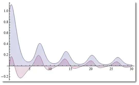
Plot both. It "makes sense". Indeed 1st solution here plays the role of sort of a driving force, so on the graphs below you see synchronization between oscillations.
Plot[{Evaluate[y[x] /. sol1], Evaluate[z[x] /. sol2]}, {x, 0, 30}, PlotRange -> All]

Now you can do more advanced things, like using also derivative of the "Interpolating Function" inside of new equations:
sol3 = NDSolve[{y'[x] == y[x] Cos[x + y[x]], y[0] == 1}, y, {x, 0, 30}];
sol4 = NDSolve[{z'[x]== -z[x]+First[y[x]/5 + y'[x] /. sol3], z[0] == 0}, z, {x, 0, 30}];
Plot[{Evaluate[y[x] /. sol3], Evaluate[z[x] /. sol4]}, {x, 0, 30},
      PlotRange -> All, Filling -> 0]