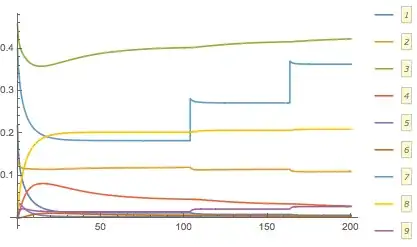
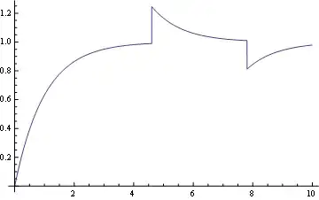
Because the equations are nonlinear, there is no assurance that equilibrium solutions even exist for a given set of k and initial conditions. However, if they do exist, an alternative, and perhaps more informative, approach is to compute them directly:
xs = Solve[Thread[Table[0, {i, Length[des[[1]]]}] == des[[2]] /. x[n_][t] -> x[n]],
     Table[x[i], {i, Length[des[[1]]]}]]
Although Solve warns
Solve::svars: Equations may not give solutions for all "solve" variables. >>
playing a bit with Reduce strongly suggests that Solve gives all the equilibrium solutions here:
{* {{x[3] -> ((k[2] + k[3]) x[5])/(k[1] x[1]),
      x[4] -> (k[3] (k[5] + k[6]) x[5])/(k[4] k[6] x[2]),
      x[6] -> (k[3] x[5])/k[6], x[8] -> (k[7] x[1] x[7])/k[8],
      x[9] -> (k[9] x[2] x[7])/k[10]},
   {x[1] -> 0, x[4] -> 0, x[5] -> 0, x[6] -> 0, x[8] -> 0, x[9] -> (k[9] x[2] x[7])/k[10]},
   {x[1] -> 0, x[2] -> 0, x[5] -> 0, x[6] -> 0, x[8] -> 0, x[9] -> 0},
   {x[2] -> 0, x[3] -> 0, x[5] -> 0, x[6] -> 0, x[8] -> (k[7] x[1] x[7])/k[8],
      x[9] -> 0}} *}
(For each of the four solutions, any x that do not appear can take any value.) With the equilibrium solutions known, one can linearize the equations des about them, Laplace transform the resulting linear equations, and Solve them to obtain the Eigensystems, completely determining the perturbed solutions in closed form.
Addendum
In answer to the question posed below in a comment, the right side of des can be linearized about an equilibrium solution without difficulty. (The left side already is linear.)
desl = Coefficient[des[[2]] /. x[n_][t] -> x[n] + e dx[n], e]

(* {dx[5] k[2] + dx[5] k[3] + dx[8] k[8] - dx[3] k[1] x[1] -
      dx[7] k[7] x[1] - dx[1] k[1] x[3] - dx[1] k[7] x[7],
    dx[6] k[5] + dx[6] k[6] + dx[9] k[10] - dx[4] k[4] x[2] -
      dx[7] k[9] x[2] - dx[2] k[4] x[4] - dx[2] k[9] x[7],
    dx[5] k[2] + dx[6] k[6] - dx[3] k[1] x[1] - dx[1] k[1] x[3],
    dx[5] k[3] + dx[6] k[5] - dx[4] k[4] x[2] - dx[2] k[4] x[4],
    -dx[5] k[2] - dx[5] k[3] + dx[3] k[1] x[1] + dx[1] k[1] x[3],
    -dx[6] k[5] - dx[6] k[6] + dx[4] k[4] x[2] + dx[2] k[4] x[4],
    dx[8] k[8] + dx[9] k[10] - dx[7] k[7] x[1] - dx[7] k[9] x[2] - dx[1] k[7] x[7] -
      dx[2] k[9] x[7],
    -dx[8] k[8] + dx[7] k[7] x[1] + dx[1] k[7] x[7],
    -dx[9] k[10] + dx[7] k[9] x[2] + dx[2] k[9] x[7]} *)
At this point, equilibrium values of x are substituted (via Rules) into the last result and the Eigenvaluess computed. These Eigenvaluess are the growth rates of the perturbations dx. (Complex Eigenvaluess indicate oscillatory solutions.) For instance, if all equilibrium values are 0, then
Eigenvalues[(CoefficientArrays[desl, Array[dx, 9]][[2]] // Normal) /.
  Thread[Array[x, 9] -> 0]]
(* {0, 0, 0, 0, 0, -k[2] - k[3], -k[5] - k[6], -k[8], -k[10]} *)
Hence, if any of k[2] + k[3], k[5] + k[6], k[8], or k[10] are negative, then perturbations grow exponentially. More generally, one would substitute one of the four equilibrium solutions xs derived earlier into the perturbed equations.
Another advantage of the procedure described here is this: In the event that an equilibrium admits exponentially growing perturbations, then attempts to solve for that equilibrium using NDSolve are likely to be unstable too.


NDSolve[ ]code – Dr. belisarius Jun 18 '15 at 16:09Subscripts, they hurt my eyes! I recommend using, for instance,x[1][t]in place ofSubscript[x,1][t], becauseSubscripts act weird in Mathematica. Also, yourinit: is this meant to be a set of initial conditions that you are feeding toNDSolve, because you should have==in place of=. Finally, please include values for your initial conditionsSubscript[T, i]. – march Jun 18 '15 at 16:17