Confusion with SplineFit (Angle calculation)

Question

This question is a continuation to [this other one][1]

I am creating polymers (where each monomer is of equal length) using this method:

num = 50;
angles = Table[RandomVariate[NormalDistribution[0, 0.2], 80], {i, 1, num}];
a1 = 1;
anglePath1[angles_, a_] := FoldList[# + a {Cos@#2, Sin@#2} &, {0, 0}, Accumulate@angles]
p1 = Table[anglePath1[angles[[i]], a1], {i, 1, num}];

Then, I use SplineFit

Needs["Splines`"];
spt = Table[SplineFit[p1[[i]], Cubic], {i, num}];
lt = Table[spt[[i]][[2, -1]], {i, num}];

Then, I break the polymer into monomers of equal length. To do so, I calculate the arc length of the polymer:

dz = .0000001;
arc = Table[
  NIntegrate[
   Norm[(spt[[i]][z + dz] - spt[[i]][z])/dz], {z, 0, lt[[i]]}, 
   MaxRecursion -> 12], {i, num}]
mesh = Table [Solve [arc[[i]]/a1 == div], {i, 1, Length[arc]}];
meshf = Flatten[Round[div /. mesh]]

After this I extract co-ordinates:

plot = Table[ParametricPlot[spt[[i]][t], {t, 0, lt[[i]]}, 
       MeshFunctions -> {"ArcLength"}, Mesh -> {meshf[[i]]}, 
       MeshStyle -> {PointSize[0.01], Red}], {i, num}];
coord = Table[
   Sort@Cases[Normal@plot[[i]], Point[p_] :> p, Infinity], {i, num}];

Now I am trying to calculate angles:

1. Using Coordinates p1

vecp = Table[Differences@p1[[i]], {i, 1, num}];
vecp2 = Table[Partition[vecp[[i]], 2, 1], {i, 1, num}];
angp = Table[VectorAngle @@@ vecp2[[i]], {i, 1, num}];
angp2 = Flatten[angp];

2.Using Coordinates coord

vecc = Table[Differences@coord[[i]], {i, 1, num}];
vecc2 = Table[Partition[vecc[[i]], 2, 1], {i, 1, num}];
angc = Table[VectorAngle @@@ vecc2[[i]], {i, 1, num}];
angc2 = Flatten[angc];

Both of these angles should have Normal Distribution (similar to the distribution of angles):

Histogram[Flatten[angles], {0.1}]

But I don't get similar distribution.
[1]: Why are these methods giving me different results? (Trying to test SplineFit)

Answer 1

The following is (I believe) a better implementation for at least two reasons. First, it doesn't use the old Splines package, but Interpolation[..., Method -> "Spline"] instead. Second, if uses an algorithmic arc length parametrization to get the equispaced points instead of relying on the mesh generated by ParametricPlot which is nice for displaying but not designed for extracting the points' coordinates from the plot.

I also modified the way you are measuring the inter-monomer angles, for the better, I think.

ClearAll[setMonomerPoints, getInterpolatingCurve, 
         getEquispacedPointsOnCurve, arcLenReparametrization];

setMonomerPoints[numberOfMonomers_, monomerLength_, angleSigma_] := 
 Module[{angles, anglePath},
  anglePath[angles_, a_] := FoldList[#+ a {Cos@#2,Sin@#2} &, {0,0}, Accumulate@angles];
  angles = RandomVariate[NormalDistribution[0, angleSigma], numberOfMonomers];
  anglePath[angles, monomerLength]
  ]

getInterpolatingCurve[pts_, interpOrder_] := Module[{prepList},
  prepList = MapIndexed[{#2[[1]], #1} &, pts];
  Interpolation[prepList, Method -> "Spline", InterpolationOrder -> interpOrder]
  ]

getEquispacedPointsOnCurve[fun_InterpolatingFunction, numberOfpoints_] :=
 Module[{cLen, dom = First@fun["Domain"], z, arcLenReparametrization, 
        eqNewCoords, eqParmRange},

  arcLenReparametrization[f_, len_] := arcLenReparametrization[f, len] =
    Module[{t, s}, NDSolveValue[{t'[s] == 1/Norm[f'[t[s]]], t[0] == dom[[1]]}, 
                                 t, {s, 0, len}]];

  (* Calculate total curve arc length *)
  cLen = NIntegrate[Norm[fun'[z]], Evaluate@{z, Sequence @@ dom}, MaxRecursion -> 12];
  (* generate numberOfpoints+1 points along the interval {0, cLen} *)
  eqParmRange = Rescale[Range[0, 1, 1/numberOfpoints], {0, 1}, {0, cLen}];
  (* Calculate the value of the function's parameter in those points *)
  eqNewCoords = arcLenReparametrization[fun, cLen][eqParmRange];
  (* calculate the position for the equispced points *)
  fun /@ eqNewCoords]

A test drive:

SeedRandom[42];
nMonomers = 80;
ss = setMonomerPoints[nMonomers, 1, .2];
f = getInterpolatingCurve[ss, 3];
eqsp = getEquispacedPointsOnCurve[f, nMonomers];
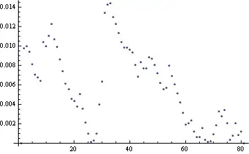
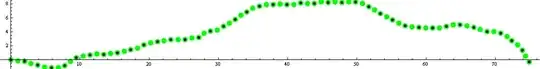
ListPlot[{ss, eqsp}, AspectRatio -> Automatic, 
         PlotStyle -> {{PointSize[.01], Green}, {PointSize[.005], Black}}]

The points look the same because the curve is smooth but it "follows" the segmented line quite well. But despite the look, they aren't the same:

ListPlot[EuclideanDistance @@@ Transpose[{ss, eqsp}]]  

Please note that if you change in the code above

eqsp = getEquispacedPointsOnCurve[f, nMonomers];

by

eqsp = getEquispacedPointsOnCurve[f, nMonomers / 2];

You'll get:

Let's generate and check the angle's statistic you're worried about. We will use the Cross product instead of VectorAngle to preserve the signs:

SeedRandom[42];
nMonomers = 80;
sigma = .2;
p1 = Table[setMonomerPoints[nMonomers, 1, sigma], {100}];
p2 = getEquispacedPointsOnCurve[#, nMonomers] & /@ (getInterpolatingCurve[#, 3] & /@ p1);
vecc2 = Partition[#, 2, 1] & /@ Differences /@ p2;
vecc3 = vecc2 /. {x : _?NumericQ, y_?NumericQ} :> {x, y, 0};
angc = ArcSin[Flatten[Map[Cross @@ #/Times @@ Norm /@ # &, vecc3, {2}][[All, All, 3]]]];
GraphicsRow[{Histogram[angc, {.01}], 
             ProbabilityPlot[angc, NormalDistribution[0, sigma]]}]

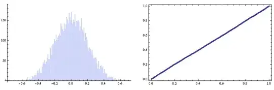
So everything looks fine enough :)

---

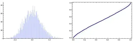
Finally a warning note: If you have a good fit for the interpolating curve but you can't estimate well the number of monomers, the statistics may go astray. Just look;

SeedRandom[42];
nMonomers = 80;
sigma = .2;
p1 = Table[setMonomerPoints[nMonomers, 1, sigma], {100}];
(* Note the "2" in the line below *)
p2 = getEquispacedPointsOnCurve[#, nMonomers/2] & /@ (getInterpolatingCurve[#, 3]&/@ p1);
vecc2 = Partition[#, 2, 1] & /@ Differences /@ p2;
vecc3 = vecc2 /. {x : _?NumericQ, y_?NumericQ} :> {x, y, 0};
angc = ArcSin[Flatten[Map[Cross @@ #/Times @@ Norm /@ # &, vecc3, {2}][[All, All, 3]]]];
GraphicsRow[{Histogram[angc, {.01}], 
             ProbabilityPlot[angc, NormalDistribution[0, sigma]]}]