DiscretizeRegion of ImplicitRegion too small

Question

I have a 2D function that has some sharp peeks within the my domain. I need to find a tight region that contains these sharp peeks. The following is an example of what I would like to do.

An example function:

Clear[f]
f[x_, y_] := 1/(1/4 + Sqrt[(x - 1)^2 + (y - 1)^2]);

Clearly this function has a max of 4 at {1,1}. I can find a region around the max via:

zmax=3.9;
R = DiscretizeRegion[ImplicitRegion[f[x, y] >= zmax, {{x, 0, 2}, {y, 0, 2}}]]

This works great but as zmax gets closer to 4.0 there comes a point where it no longer works like at zmax=3.999

Is there a way I can help ImplicitRegion and/or DiscretizeRegion to know where to look? In my real problem I start with a zmax that works and loop through larger and larger values for zmax. I have done a FindMaximum so I know how far I can go. I would like to do something like the following which does not work:

zmax=3.9;
R = DiscretizeRegion[ImplicitRegion[f[x, y] >= zmax, {{x, 0, 2}, {y, 0, 2}}]];

rm = RegionMember[R];

zmaxmax=3.999;
R = DiscretizeRegion[ImplicitRegion[f[x, y] >= zmaxmax && rm[{x,y}], {{x, 0, 2}, {y, 0, 2}}]];

Where I would like to use what I have learned in my last step to inform my next step. But sadly this does not work.

Answer 1

Your original approach can work if you exploit RegionPlot as an alternative to DiscretizeRegion. With RegionPlot, the resulting Graphics must be deconstructed to find the corresponding region. However, you can use the PlotPoints option to offer some help finding small regions.

I thought the Method->"RegionPlot" option of DiscretizeRegion might be used to accomplish the same thing, but I can’t see how to pass a PlotPoints sub-option to it. So instead, here’s a function that spells it all out.

ClearAll[newDiscretizeRegion];

Options[newDiscretizeRegion] = {PlotPoints -> 40};

newDiscretizeRegion[region_, {{xMin_, xMax_}, {yMin_, yMax_}}, OptionsPattern[]] := 
    Module[
       {graphics, points, boundary, mesh},

       graphics = RegionPlot[
         {x, y} \[Element] region, {x, xMin, xMax}, {y, yMin, yMax},
         PlotPoints -> OptionValue[PlotPoints]
       ];
       points = FirstCase[graphics, _GraphicsComplex, Null, Infinity][[1]];
       boundary = FirstCase[graphics, _Line, Null, Infinity];
       mesh = First@Normal@GraphicsComplex[points, boundary/.Line->Polygon];
       DiscretizeRegion@mesh
    ];

Note that the PlotPoints option defaults to 40. Use a larger value if the region is still not found or to get added resolution in the result. This could be made more automatic, of course.

With this function, your approach would look something like this. Here the PlotPoints option is gradually increased, but it can be profiled differently for better speed. The final value (220 in this example) determines how smooth the mesh boundary will be.

ClearAll[f];

f[x_, y_] := 1/(1/4 + Sqrt[(x - 1)^2 + (y - 1)^2]);

ClearAll[deltaGoal, bounds, nextzmax, zmax, plotPoints, R];

deltaGoal = 1*^-12;
bounds = {{0, 2}, {0, 2}};
nextzmax = 3;
plotPoints = 40;

While[4 - nextzmax > deltaGoal,
  zmax = nextzmax;
  R = newDiscretizeRegion[ImplicitRegion[f[x, y] >= zmax, {x, y}], bounds, 
    PlotPoints -> plotPoints];
  bounds = RegionBounds[R, "Sufficient"];
  nextzmax = 4 - 0.1 (4 - zmax);
  plotPoints += 15;
  ];

Print[{InputForm@zmax, InputForm@bounds}];
R

 

{3.999999999999], {{0.9999999999999345, 1.000000000000066},{0.9999999999999345, 1.000000000000066}}]}

I haven't tried to extend this for functions with multiple peaks, which you would have to find and isolate before iterating as indicated.

Answer 2

Here's a way that takes advantage of the undocumented PlotPoints form that allows specific sample points to be included. See Specific initial sample points for 3D plots for more.

Test function

I'll construct a function with five maxima of the same height.

SeedRandom[0];
ncp = 5;
cp = RandomReal[{0, 2}, {ncp, 2}];

f[x_, y_] = Simplify[     (* set up with unknown coefficients C[1], C[2],... *)
   Sum[C[i]/(1/4 + EuclideanDistance[{x, y}, cp[[i]]]), {i, ncp}],
   {x, y} ∈ Reals];
f[x_, y_] = f[x, y] /.    (* solve for the coefficients *)
    First@Solve[Equal @@@ Partition[f @@@ cp, 2, 1], Array[C, ncp - 1]] /.
     C[ncp] -> 1;

f @@@ cp
(*  {7.25243, 7.25243, 7.25243, 7.25243, 7.25243}  *)

Discretizing RegionPlot

Sometimes it's just easier to build things up from plots that to use the region functionality. (I expect this to improve, since WRI does pay attention to how users use Mathematica and adapts its interfaces to suit common usage.)

max = f @@ First[cp] - 0.001;
reg = DiscretizeGraphics@
   RegionPlot[f[x, y] > max, {x, 0, 2}, {y, 0, 2}, PlotPoints -> {Automatic, cp}];

The regions are minuscule, so I made the boundaries thick enough to see.

HighlightMesh[reg, Style[1, Red, Thick]]

A check. I had to exaggerate the max level to max - 0.2 to get a visible result. The regions are just too small for screen resolution.

Plot3D[f[x, y], {x, 0, 2}, {y, 0, 2}, MeshFunctions -> {#3 &}, 
 Mesh -> {{max - 0.2}}, MeshShading -> {Automatic, Red}, 
 PlotPoints -> {Automatic, cp}, MaxRecursion -> 3]

Alternative for higher quality

I'm not sure what the use-case is. The regions produced above, if you zoom in on them, are very blocky and often square. If high-resolution regions are required, then RegionPlot is an expensive way to go. An alternative is to use implicitCurve from my answer to Getting an InterpolatingFunction from a ContourPlot to get a parametrization of the curve f[x, y] == max and use it to construct a polygon. We can also adapt periodicEvent from my answer to Plotting implicitly-defined space curves to 2D to detect when we've traced the entire loop around each maximum. Beware: Region functionality is as yet only available at MachinePrecision. Even though, implicitCurve can be used with high WorkingPrecision, there are limits to how far it can be used to create high-precision regions.

The function

nbhdBoundaries[fn, level, cps]

uses implicitCurve to solve the equation fn == level in the neighborhood of each critical point in the list cps. It returns a list of parameterizations of the boundaries. Each parametrization is a pair of the form

{x -> InterpolatingFunction[<>], y -> InterpolatingFunction[<>]}

The function

discretizeParametricLoop[{x -> InterpolatingFunction[<>], y -> InterpolatingFunction[<>]}]

takes such a pair and returns a MeshRegion of the region contained by the parameterization. (Code at bottom.)

Here are the functions applied to the example above:

reg = RegionUnion @@
   DiscretizeRegion /@ discretizeParametricLoop /@ nbhdBoundaries[f[x, y], max, cp];
HighlightMesh[reg, Style[1, Red, Thickness[0.01]]],

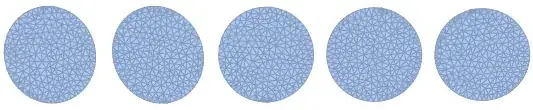
Here are the individual regions:

Show /@ DiscretizeRegion /@ 
   discretizeParametricLoop /@ 
    nbhdBoundaries[f[x, y], max, cp] // GraphicsRow

Code dump:

Note that the starting value for the point in implicitCurve is neither checked nor adjusted for satisfying the equation eqn. If it is not on the curve, what will happen is that a different level curve will be returned. (Checking is not hard to add; adjusting and finding can in general be tricky.)

ClearAll[implicitCurve, periodicEvent]

variableQ = Quiet@ListQ@Solve[{}, #] &;

(* creates a WhenEvent to stop integration when variables return to their initial values *)
periodicEvent[
   vars : {x_?variableQ, ___?variableQ}, 
   p0 : {x0_?NumericQ, ___?NumericQ},
   tolerance_: 0.01] := 
  WhenEvent[x == x0 && Norm[vars - p0] < tolerance, "StopIntegration"];

Options[implicitCurve] = Join[{"Events" -> {}}, Options[NDSolve]];
implicitCurve[
   eqn_,                                                (* equation to paramterize *)
   {x_?variableQ, x0_?NumericQ},                        (* x & starting value *)
   {y_?variableQ, y0_?NumericQ},                        (* y & starting value *)
   {tmin_?NumericQ, tmax_?NumericQ | tmax : Infinity},  (* integration interval *)
    opts : OptionsPattern[]] := Module[{t, ode},
   ode = {x'[t]^2 + y'[t]^2 == 1,     (*unit speed*)
     {x[0], y[0]} == {x0, y0},        (*starting point*)
     {x'[0], y'[0]} == 
      Normalize@                      (*starting direction*)
       Cross[D[eqn /. Equal -> Subtract, {{x, y}}] /. 
         Thread[{x, y} -> {x0, y0}]]};
   First@NDSolve[{eqn /. {x -> x[t], y -> y[t]}, ode, 
      OptionValue["Events"] /. {x -> x[t], y -> y[t]}}, {x, y}, {t, 
      tmin, tmax}, FilterRules[{opts}, Options[NDSolve]]]];

In nbhdBoundaries we have to knock the initial search point for FindRoot off of the critical point, probably because the gradient is singular; in any case, FindRoot did not work reliably using the critical point as the initial point. The offset dy assumes the function does not vary wildly, as in the test function. I used the minimum distance between the critical points as a scale. The secant line method (replace {y, Last[cp] + dy} by {y, Last[cp], Last[cp] + dy}) might be more robust or the scale might need to be adjusted in some cases.

ClearAll[nbhdBoundaries, discretizeParametricLoop];
nbhdBoundaries[fn_, level_, cps_] := Module[{x0, y0, dy},
   dy = Min[EuclideanDistance @@@ Subsets[cp, {2}]]/100;
   Function[{cp},
     x0 = First[cp];      (* find starting point on curve *)
     y0 = y /. FindRoot[fn == level /. x -> x0, {y, Last[cp] + dy}];
     implicitCurve[       (* integrate the parametrization *)
      f[x, y] == level,
      {x, x0},
      {y, y0},
      {0, Infinity},
      "Events" ->         (* stops the integration after one loop *)
        {periodicEvent[{x, y}, {x0, y0}, EuclideanDistance[cp, {x0, y0}]/10]}
      ]
     ] /@ cps];

discretizeParametricLoop[{_ -> xif_, _ -> yif_}] :=
  Polygon[Transpose[{xif["ValuesOnGrid"], yif["ValuesOnGrid"]}]];

An alternative discretizeParametricLoop, that uses ParametricPlot to give a smoother boundary:

discretizeParametricLoop[{_ -> xif_, _ -> yif_}] := Block[{t},
   First@Cases[
     ParametricPlot @@ {{xif[t], yif[t]}, Flatten@{t, xif["Domain"]}},
     Line[p_] :> Polygon[p],
     Infinity]
   ];