Using codes to replicate drawing tools in Mathematica

Question

This might seem very obvious but I'm on the verge of losing all the annotations I've made on a graph because I can't figure a way to save it after using the drawing tool to add a few extras to the graph. Each time I save the graph, the texts become illegible. Any help would be really appreciated. I've tried highlighting and saving, i've also tried right clicking and saving as graphics-same results. Difficult to give a reproducible example here. Is there a way to invoke the drawing tools using codes?

Here's some code to work with:

Labeled[Plot[-x^2 - 4, {x, 0, 5}, ImageSize -> 500, 
AxesOrigin -> {0, -1}], {"Y axis", "X Axis"}, {Left, Top}, 
RotateLabel -> True]

For example, I'd like to replicate an image similar to this (without the grid): quadratic equation

just insert a new variable before the graphic en evaluate:
gra=modifiedGraphic — elbOlita, Jul 02 '15 at 18:09
Thanks for you comment. This doesn't seem to be working-each time I try to save it as the new graph, it produces the previous one. Could you clarify a bit further? — John_dydx, Jul 02 '15 at 18:15
hard to explain as you mentioned. but see this https://drive.google.com/file/d/0B_XdZgJpywbRTXZfNmt1WDY2N00/view?usp=sharing — elbOlita, Jul 02 '15 at 18:25
Thanks, I think that method works on purely drawing but if you try to produce a plot in mathematica and then label it and then save it, it doesnt seem to work. Perhaps try to draw on the graph in my post (edited) and then save and see if it works. — John_dydx, Jul 02 '15 at 18:31
Select cell then use File | Save Selection As ... then Import[<file pathname>] Use Insert | File Path... to get <file pathname> — Bob Hanlon, Jul 02 '15 at 18:45
@BobHanlon, thanks for your comment. So you mean I should first save the annotated graph and then import into mathematica. Why do I need to import again? I only want to save in as a pdf-I've tried this but the saved graph comes out wrong-very large axes labels with some bits cut off. — John_dydx, Jul 02 '15 at 18:52
Your question merely asked for a way to save the annotated plot so as not to lose the annotations. The Import is just to demonstrate that the plot is saved with the annotations. Pick whatever format (.jpg, .png, .pdf, ...) gives you the best results for your purpose. If you want the notebook to be able to regenerate the annotated plot, add the annotations with Epilog using graphic primitives. — Bob Hanlon, Jul 02 '15 at 19:12
Why are you labeling you axes with labeled? It would be much easier to use AxesLabel->{x,y} inside the plot function. And yes, you are right, my method wont work with Labeled graphic — elbOlita, Jul 02 '15 at 19:35
@elbOlita, pls see my previous post-http://mathematica.stackexchange.com/questions/87388/positioning-axes-labels — John_dydx, Jul 02 '15 at 19:39
@BobHanlon, thanks. The annotation on the plot is preserved but for some reason the axes labels are illegible in the saved version. I guess Mathematica is not the best tool for this job. — John_dydx, Jul 02 '15 at 19:40
A way that I personally find much better is not to use a drawing tool, but to make all things programmatically. It is just for the reason that exactly 5 minutes after I have finished the modifications of the graph, I get a new idea of what should be added to it. Programmatic drawing is astonishingly easy. It is based on the Show statement unifying different elements. I suggest that if you edit your question by adding to it an image of what you are after, I might give a possible code. — Alexei Boulbitch, Jul 03 '15 at 06:49
@AlexeiBoulbitch, thanks for your comment. I would love to have a go at it using codes, I'll attach similar image to what I'm after in my original post. Cheers. — John_dydx, Jul 03 '15 at 08:04

score 7 · Accepted Answer · answered Jul 03 '15 at 10:36

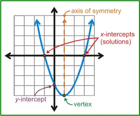
Just to give the initial idea, this is the code drawing most of the picture in question:

 Manipulate[
 Show[{
   Plot[4 (z - 0.5)^2 - 3, {z, -1, 2}, PlotRange -> {-3.5, 2.2}, 
    Ticks -> None, AxesStyle -> Arrowheads[{-0.03, 0.03}]],
   Graphics[{Orange, Dashed, Thickness[0.008], Arrowheads[0.05], 
     Arrow[{{0.5, -3}, {0.5, 2}}]}],
   Graphics[{Text[Style["Axis of symmetry", 12, Orange], 
      Scaled[{0.7, 0.97}]], 
     Text[Style["x-intercepts", 12, Red], Scaled[{0.8`, 0.218`}]]}],
   Graphics[{Orange, Thickness[0.002], 
     Arrow[{Scaled[{0.62, 0.934}], Scaled[{0.504`, 0.78}]}]}],
   Graphics[{Red, PointSize[0.02], Point[{-0.366, 0}], 
     Point[{1.366, 0}]}],
   Graphics[{Red, Thickness[0.002], 
     Arrow[{Scaled[{0.8`, 0.25}], Scaled[{0.78`, 0.59`}]}], 
     Arrow[{Scaled[{0.8`, 0.25}], Scaled[{x, y}]}]}]      
   }], {x, 0, 1}, {y, 0, 1}]

That is what you should see on the screen:

enter image description here

Now, some explanations.

The main statement is Showwrapping the whole drawing.
The latter consists of the Plot drawing the parabola along with axes specification on one hand and several Graphics statements on the other hand. These draw arrows, text labels and so on.
The whole code is wrapped by the Manipulatestatement. This is technical. Manipulate is used, while the drawing is being done to rapidly find various coordinates. The example is given directly in the code, where I specified the end coordinates of the second red arrow by the dynamically varying coordinates x and y. One finds x and y by moving the sliders, and copy-pastes the corresponding values into the code. Just play with them.

By the same procedure it is easy to draw other elements of your target picture.

After the drawing is finalized, remove the manipulate statement. Done.

The last thing, is that if you need to have bent arrows indicating the characteristic points, you might want to use Bezier curves instead of arrows.

Have fun!

Wow, this is the work of a genius! Simply brilliant! Thanks so much. — John_dydx, Jul 03 '15 at 11:38
Thanks once again. I've managed to produce the plot I wanted using your codes. — John_dydx, Jul 03 '15 at 17:05

score 2 · Answer 2 · edited Jul 08 '16 at 02:30

I had a similar problem to "I can't figure a way to save it after using the drawing tool to add a few extras to the graph. Each time I save the graph, the texts become illegible"

A solution that worked for me is as follows

a) Make all changes using DrawingTools

b) Copy this figure (using Command-C if you wish) and equate this to a new name e.g. figtemp= paste (using Command-V)

c) At this point you can verify that by typing figtemp, MMA reproduces the edited figure you wish to export.

d) Now you can save or, most preferably (due to compactness) export the figure using the Export command wrapped around figtemp

All the best

Using codes to replicate drawing tools in Mathematica

2 Answers2