I have some data set that I am trying to find the maximums . I figured I could do this by fitting the many peaks of the dataset to Gaussian distributions and then finding the peaks of this data from these fit functions:
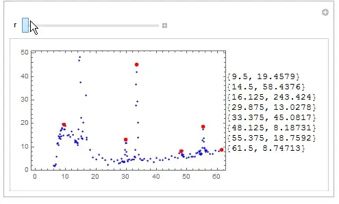
data = {{6, 2.1}, {6.25, 1.82394}, {6.5, 2.056}, {6.75, 2.48818}, {7,
  5.73034}, {7.25, 11.3611}, {7.5, 11.5297}, {7.625, 10.6597}, {7.75,
  14.5473}, {7.875, 13.7337}, {8, 14.291}, {8.125, 15.4141}, {8.25,
  13.2849}, {8.375, 16.785}, {8.5, 14.6091}, {8.625, 17.0505}, {8.75,
  17.9138}, {8.875, 17.662}, {9, 19.6648}, {9.125, 14.9366}, {9.25,
  19.6298}, {9.375, 17.377}, {9.5, 19.4579}, {9.75, 17.3271}, {10,
  19.0673}, {10.5, 14.7837}, {11, 15.2593}, {11.5, 14.2707}, {12,
  16.7271}, {12.5, 15.0264}, {13, 12.8453}, {13.125, 11.8129}, {13.25,
   12.2551}, {13.375, 12.4764}, {13.5, 12.3054}, {13.625,
  12.2718}, {13.75, 11.7467}, {13.875, 11.6148}, {14,
  10.7611}, {14.125, 13.5223}, {14.25, 17.3761}, {14.375,
  46.9357}, {14.5, 58.4376}, {14.625, 57.7595}, {14.75,
  48.2346}, {14.875, 37.6358}, {15, 22.366}, {15.125,
  14.6147}, {15.25, 13.7916}, {15.375, 13.6754}, {15.5,
  13.483}, {15.625, 16.7153}, {15.75, 20.2869}, {15.875,
  81.1927}, {16, 231.151}, {16.125, 243.424}, {16.25,
  232.654}, {16.375, 181.878}, {16.5, 111.372}, {16.625,
  64.9912}, {16.75, 32.0148}, {16.875, 13.9479}, {17, 13.0599}, {18,
  8.65011}, {19, 5.44097}, {20, 4.66879}, {21, 6.56693}, {22,
  5.12372}, {23, 4.34006}, {24, 2.44913}, {25, 4.56596}, {26,
  3.78848}, {27, 4.33847}, {27.5, 2.89337}, {28, 3.12278}, {28.5,
  5.02059}, {28.625, 3.68042}, {28.75, 3.90491}, {28.875,
  3.68717}, {29, 3.57609}, {29.125, 3.35689}, {29.25,
  3.46561}, {29.375, 3.91997}, {29.5, 6.82568}, {29.625,
  8.61445}, {29.75, 11.7729}, {29.875, 13.0278}, {30,
  11.555}, {30.125, 7.86307}, {30.25, 6.16789}, {30.375,
  4.26774}, {30.5, 3.93371}, {31, 4.59788}, {31.5, 4.49401}, {32,
  4.71784}, {32.5, 4.71958}, {32.625, 5.72564}, {32.75,
  5.94579}, {32.875, 5.49908}, {33, 8.74719}, {33.125,
  27.7096}, {33.25, 36.5386}, {33.375, 45.0817}, {33.5,
  42.019}, {33.625, 29.3559}, {33.75, 20.2754}, {33.875,
  14.0957}, {34, 6.77348}, {34.5, 5.07823}, {35, 4.40521}, {35.5,
  4.40848}, {36, 4.86514}, {37, 4.18628}, {38, 4.98291}, {39,
  3.62528}, {40, 5.21134}, {41, 4.4216}, {42, 4.42242}, {43,
  5.32562}, {44, 4.54088}, {45, 6.24023}, {46, 5.45007}, {47,
  5.11135}, {47.5, 7.20017}, {48, 7.94951}, {48.125, 8.18731}, {48.25,
   6.37029}, {48.375, 6.95074}, {48.5, 8.55079}, {48.625,
  6.38578}, {48.75, 6.7367}, {48.875, 5.8178}, {49, 5.82325}, {50,
  5.36753}, {50.5, 5.60118}, {51, 6.97421}, {51.5, 5.71228}, {52,
  5.83199}, {52.5, 5.84295}, {53, 7.32958}, {53.5, 7.6847}, {54,
  8.02426}, {54.125, 6.88053}, {54.25, 7.81263}, {54.375,
  6.66246}, {54.5, 8.50358}, {54.625, 6.55995}, {54.75,
  7.37252}, {54.875, 6.91174}, {55, 9.66547}, {55.125,
  12.6715}, {55.25, 17.5031}, {55.375, 18.7592}, {55.5,
  13.7057}, {55.625, 12.2038}, {55.75, 9.21217}, {55.875,
  9.67643}, {56, 8.55033}, {56.125, 8.7981}, {56.25, 7.869}, {56.375,
  8.46045}, {56.5, 8.34932}, {57, 7.9999}, {57.5, 7.07507}, {58.5,
  6.97235}, {59.5, 8.48789}, {60.5, 8.03506}, {61.5, 8.74713}}

counts=data[[All,2]]
Then I attempt to find the fits to the peaks of this data, which should be a distribution made up of many NormalDistribution functions:
nd =
  FindDistribution[counts,
    TargetFunctions -> {NormalDistribution}]
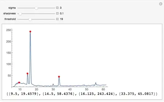
However, This results in the following distribution:
0.000599601 E^(-0.0000772966 (-91.0024 + x)^2) +
 0.0712972 E^(-0.0206633 (-9.10869 + x)^2)
The following plot of this distribution:
Show[Plot[
  0.0005996013554770311` E^(-0.00007729656053053849` \
(-91.00239606190587` + x)^2) +
   0.07129715654128815` E^(-0.020663257993617158` \
(-9.108687446977836` + x)^2), {x, 0, 60}],
 ListPlot[data]]
Does not fit my data very well. Any suggestions on how to output the many Normal distributions that fit the peaks of my data set?