A particular contour does not show up, even though it is in my list

Question

Consider:

f = Sqrt[9 - x^2 - y^2];
ContourPlot[f, {x, -4, 4}, {y, -4, 4},
 Contours -> {0, 1, 2, 3},
 ContourLabels -> All,
 ContourShading -> None]

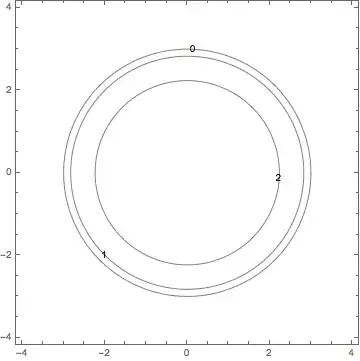
Which produces this image:

enter image description here

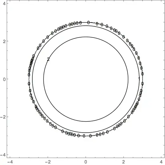
Now, I understand that the contour f=3 is just the point (0,0) and maybe that's why it's not drawn. But I don't understand why the contour f=0, which should be a circle of radius 3, is missing?

Any thoughts?

@EnriquePérezHerrero 9 - x^2 - y^2 /. {x -> 3/Sqrt@2, y -> 3/Sqrt@2} — Dr. belisarius, Jul 08 '15 at 19:23
@EnriquePérezHerrero: When finding the contour $f=0$, we're working with $\sqrt{9-x^2-y^2}=0$, which is equivalent to $x^2+y^2=9$, which is a circle of radius 3. We are not substituting 3 for $x$ and $y$. But see Michael Seifert's answer. But thanks for the reply. — David, Jul 08 '15 at 20:05
@Mr.Wizard My plotting badge means my single vote would close it. I would rather someone (or two) agree first. — Michael E2, Jul 09 '15 at 03:56
@MichaelE2 Sorry, I completely forgot about gold badge closes; I do the same thing. I agree that this seems to be a duplicate of 23363; if that's good enough for you I suggest you go ahead and close it. — Mr.Wizard, Jul 09 '15 at 05:25

Michael Seifert · Accepted Answer · 2015-10-21T15:32:30.070

6

It appears to be a problem with the square root:

f = 9 - x^2 - y^2;
ContourPlot[f, {x, -4, 4}, {y, -4, 4}, Contours -> {0, 1, 4, 9}, 
 ContourLabels -> (Text[Sqrt[#3], {#1, #2}] &), ContourShading -> None]

enter image description here

My guess is that the algorithm used by ContourPlot implicitly relies on the function having a smooth gradient in some neighborhood of each contour, which the function $f = \sqrt{9 - x^2 - y^2}$ does not have in the neighborhood of the level set $f = 0$.

edited Oct 21 '15 at 15:32

answered Jul 08 '15 at 19:29

Michael Seifert

15,208
31
68

Probably a good point. Thanks for the help. – David Jul 08 '15 at 19:53

Bob Hanlon · Answer 2 · 2015-07-08T20:33:21.600

f = Sqrt[9 - x^2 - y^2];

Reduce[f == 0, {x, y}, Reals]

-3 <= x <= 3 && (y == -Sqrt[9 - x^2] || y == Sqrt[9 - x^2])

Mathematica has a hard time finding a real solution for f == 0. Using a large number of PlotPoints and forcing the result to be real using Re produces a highly segmented plot (multiple labels for 0)

ContourPlot[Re[f], {x, -4, 4}, {y, -4, 4}, Contours -> {0, 1, 2, 3},
 ContourLabels -> All,
 ContourShading -> None,
 PlotPoints -> 201]

enter image description here

For a workaround use RegionPlot:

Row[{
  RegionPlot[
   ImplicitRegion[
      Reduce[
       Sqrt[9 - x^2 - y^2] == #, {x, y}, Reals],
      {x, y}] & /@
    Range[0, 3],
   PlotRange -> {{-4, 4}, {-4, 4}},
   ImageSize -> 360],
  LineLegend[
   {Red, Darker[Green], Orange, Blue},
   Range[3, 0, -1]]}]

enter image description here

A particular contour does not show up, even though it is in my list

2 Answers2