How to obtain the area enclosed by such a curve?

Question

The desired curve is defined as curve02 below :

ClearAll["Global`*"];
R = 48.78;
r = 8.13;
z1 = R/r;
z2 = 1 - z1;
e = 7.05;
f = r/e;
re = 12.6;
θ = ArcTan[Sin[z1 τ]/(f + Cos[z1 τ])] - τ;
φ = ArcSin[f Sin[θ + τ]] - θ;
ψ = z1/(z1 - 1) φ;
curve01 = {(R - r) Sin[τ] + e Sin[z2 τ] - 
     re Sin[θ], (R - r) Cos[τ] - e Cos[z2 τ] + 
     re Cos[θ]} // FullSimplify;
curve02 = {curve01[[1]] Cos[φ - ψ] - 
     curve01[[2]] Sin[φ - ψ] - e Sin[ψ], 
    curve01[[1]] Sin[φ - ψ] + 
     curve01[[2]] Cos[φ - ψ] - e Cos[ψ]} // 
   Simplify;
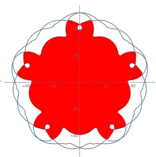
ParametricPlot[Evaluate[curve02], {τ, 0, 5 π}, 
 Exclusions -> None, MaxRecursion -> 15, PlotPoints -> 1000]

which can be visualized as:

enter image description here

How to obtain the area of its enclosed region? update

Green's theorem can solve another similar problem with high accuracy but does not suit this one, below is an example:

I tried to rewrite your original curve as below, just in order to make sure the derivatives of the parametric form can be obtained by Mathematica by avoiding Abs or Sign:

ncurve={(Cos[t]^2 )^(1/4),(Sin[t]^2)^(1/4)}

Then the numerical result of the closed area can be obtained by applying Green's theorem:

4*Quiet@NIntegrate[ncurve[[1]] D[ncurve[[2]], t], {t, 0, Pi/2}] // 
 NumberForm[#, 15] &

which gives:

3.708149351621483

score 5 · Accepted Answer · edited Apr 13 '17 at 12:55

5

Do you wan the entire area enclosed by the outer envelope? A bit brute force, but note the 10-fold symmetry, so that only two arc segments define the outer boundary:

base = Line@Table[ curve02, {\[Tau], 0, 5 Pi, Pi/1000}];
r1 = FindRoot[ (curve02 /.  \[Tau] -> x) == (curve02 /.  \[Tau] -> 
   y), {x, .5}, {y, 5.5}];
p1 = y /. FindRoot[ (ArcTan @@ (curve02 /. \[Tau] -> y)) == 
3 Pi/ 10 , {y, .55}]
top = x /. FindRoot[ curve02[[1]] /.  \[Tau] -> x , {x, 5}];
arc = Join[Table[ curve02 , {\[Tau], top, y /. r1 , .0001}], 
   Table[ curve02 , {\[Tau], x /. r1, p1 , .0001}]];
   Graphics[{base, {Red, 
         Line[{curve02 /. \[Tau] -> top, {0, 0}, curve02 /. \[Tau] -> p1}], 
         Line@arc }}]

enter image description here

now the area of the polygon slice: ( by 10 gives the total ) (https://mathematica.stackexchange.com/a/22587/2079 )

PolygonSignedArea[pts_?MatrixQ] := Total[Det /@ Partition[pts, 2, 1, 1]]/2;
area = 10 PolygonSignedArea[Reverse@Join[{{0, 0}}, arc]]

7936.86

as noted in the comments, if we set the increment to 10^-6 this converges to the more sophisticated NIntegrate result of 7945.5

edited Apr 13 '17 at 12:55

Community

1

answered Jul 17 '15 at 22:44

george2079

38,913
1
43
110

1

I got 7945.52, but I used NIntegrate. – Michael E2 Jul 17 '15 at 23:23
hi, @MichaelE2 would you please post your answer here? – LCFactorization Jul 18 '15 at 00:21
If there is a way for round off error analysis that would be great. For example, both the two answers, 7936.86 and 7945.52, which one is closer to the true area, and is there a rough upper limit estimation? – LCFactorization Jul 18 '15 at 00:27
2

@LCFactorization Using george's setup, 5 (NIntegrate[-First[curve02] D[Last@curve02, \[Tau]] + Last[curve02] D[First@curve02, \[Tau]], {\[Tau], top, y /. r1}] + NIntegrate[-First[curve02] D[Last@curve02, \[Tau]] + Last[curve02] D[First@curve02, \[Tau]], {\[Tau], x /. r1, p1}]). My brute-force approach was similar and not distinctive enough to justify a separate answer. – Michael E2 Jul 18 '15 at 00:34
2

@LCFactorization Each arc segment spans a convex wedge and any polygonalization (with vertices on the arc and origin) will underestimate the area. – Michael E2 Jul 18 '15 at 00:58
@george2079 very nice and instructive +1 – ubpdqn Jul 18 '15 at 02:04
1

@MichaelE2 thank you for instructive supplemental code snippet. – ubpdqn Jul 18 '15 at 02:05
@george2079 One more issue, the variable base in the code remains undefined. – LCFactorization Jul 18 '15 at 03:37
1

bugger. base is the original graphic, something like Line@Table[ curve02 , {\[Tau], 0,5 Pi , .01}] (or use parametric plot ). – george2079 Jul 18 '15 at 13:54
1

you might play with the discretization (.0001) to check that this converges to the NIntegrate result. – george2079 Jul 18 '15 at 13:58
thank you @ george2079 and @ MichaelE2 – LCFactorization Jul 19 '15 at 05:06

score 3 · Answer 2 · answered Jul 17 '15 at 13:07

I may have missed the point but I post out of interest.

p = ParametricPlot[curve02, {\[Tau], 0, 5 Pi}]
c[t_] := curve02 /. \[Tau] -> t
point = SortBy[c /@ Range[0, 5 Pi, 0.001], Norm];
Manipulate[
 ListPlot[point[[1 ;; n]], AspectRatio -> Automatic], {n, 1, 15000, 
  1}]

enter image description here

The manipulate allows to get "interior"

Getting desired points:

points = point[[1 ;; 9473]];
pnts = DeleteCases[
  points, {x_, y_} /; 
   Norm[{x, y}] > 
     45 && (Pi/5 < ArcTan[x, y] < Pi/2.5 || 
      Pi/5 < ArcTan[-x, y] < Pi/2.5 || 0 < ArcTan[-x, -y] < Pi/6 || 
      Pi/2.5 < ArcTan[-x, -y] < Pi/2 || 
      Pi/2.5 < ArcTan[x, -y] < Pi/2 || 0 < ArcTan[x, -y] < Pi/6)]

then

pg = Polygon[pnts[[Last@FindShortestTour[pnts]]]];
Show[p, Graphics[{Red, pg}]]
Area[pg]

where area yields: 5242.29

enter image description here

thanks. Two issues: (1). The desired area is the enclosed region by the profile of the photo, not the red; (2). how do you obtain the magic number 9473, and the logic expression for selecting desired points? — LCFactorization, Jul 17 '15 at 14:06
@LCFactorization re:(1) I am sorry I am not sure I understand your desired region (2) I used manipulate to get as close to 'interior' for step size I chose then deleted 'outside' to allow polygon...in my Timezone it is midnight so am off to sleep. Good luck :) — ubpdqn, Jul 17 '15 at 14:12

How to obtain the area enclosed by such a curve?

2 Answers2

Linked