What will happen if I set ExclusionsStyle for points in 2D plot?

Question

For example

f[x_] := (x^5 - 4 x^2 + 1)/(x - 1/2);
Plot[f[x], {x, -1, 2}, Exclusions -> {f[x] == 0}, ExclusionsStyle -> Dashed]

Has the ExclusionsStyle -> Dashed option done anything here?

Answer 1

Note: The Exclusions option is updated in v11.0, since then an additional vertical line at the singularity x == 1/2 is shown in the plot when ExclusionsStyle -> Dashed is added, so you'll find the output of samples in this answer slightly different nowadays, but this doesn't influence the conclusion.

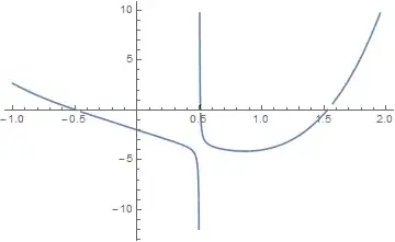
Outwardly, the graph looks just the same as the one without ExclusionsStyle -> Dashed:

f[x_] := (x^5 - 4 x^2 + 1)/(x - 1/2);
g1 = Plot[f[x], {x, -1, 2}, Exclusions -> f[x] == 0]

But it's surprising that ExclusionsStyle does make a difference actually. Let's check the graphs with Alexey Popkov's shortInputForm:

g1 // shortInputForm

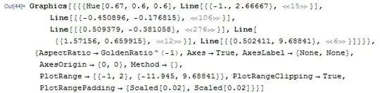
g2 = Plot[f[x], {x, -1, 2}, Exclusions -> f[x] == 0, ExclusionsStyle -> Dashed] 
g2 // shortInputForm

We can see that in both cases Exclusions breaks the curves at f[x] == 0, but when setting ExclusionsStyle -> Dashed, 3 very short dashed lines are created!

It'll be more interesting if you extend these lines with the InfiniteLine in v10:

Show[g2, Epilog -> {Red, PointSize@Medium, Point[{x, 0} /. NSolve[f[x], Reals]]}] /. 
Line[{a_, b_}] :> InfiniteLine[{a, b}]

The dashed lines seem to be tangent lines at those excluded points!

Let's check the slopes of the short lines:

Cases[g2, Line[{p1_, p2_}] :> (#2/# & @@ (# - #2) &[p1, p2]), Infinity] // Sort
(* {-449.031, -4.26733, 14.6531} *)

They're very close to the derivatives at the exclusive points:

f'[x] /. NSolve[f[x] == 0, x, Reals] // Sort
(* {-443.273, -4.26733, 14.6531} *)

Further check shows that the end points of the short lines are all on the curve:

Cases[g2, Line[{p1_, p2_}] :> (f@# - #2 & @@@ {p1, p2}), Infinity]
(* {{0., 0.}, {0., 0.}, {0., 0.}} *)

So the short lines are probably short secant lines near the exclusive points, which can be used as approximate tangent lines.

This is not the end of the analysis, m-goldberg's answer shows that the working mechanism of ExclusionsStyle is even more subtle than what I've represented in this answer, but since my original intention is just to demonstrate the interesting behavior above, I'd like to stop here at this moment.

Answer 2

I think that I stated this before in a previous post: ExclusionsStyle is a rather strange option. It works differently than other style options and the documentation on it must be read carefully.

The relevant part of the documentation for this question is that concerning the style specification for the exclusion boundary points. In the OP's example, where the excluded regions are drawn as dashed lines, only a boundary point style specification will a strong visible effect on the exclusions generated by the plot in question. The dashed lines are too short to show up at the scale of the plot.

f[x_] := (x^5 - 4 x^2 + 1)/(x - 1/2);
Plot[f[x], {x, -1, 2}, 
  Exclusions -> f[x] == 0, ExclusionsStyle -> {Dashed, Red}] 

Of course, the exclusion regions can be made visible. Here I do it in a rather gross way, just to make the point.

Plot[f[x], {x, -1, 2},
  Exclusions -> f[x] == 0, ExclusionsStyle -> {{Green, Thickness[.1]}, Red}]