VectorPlot only shows dots

Question

I am trying to plot a electric field: vec = 1/(16 π ) Abs[{ex, ey, ez}]^2;

ex = -I A (Subscript[I, 0] + Subscript[I, 2 ] Cos[ϕ]);
ey = -I A Subscript[I, 2] Sin[2 ϕ];
ez = -2 A Subscript[I, 1 ] Cos[ϕ];  

with my A=141.20 and Intensities:

Subscript[I, 0] = NIntegrate[Sqrt[Cos[θ]] Sin[θ] (1 + Cos[θ]) 
                            BesselJ[0, (v Sin[θ])/Sin[α]] 
                            Exp[I  u Cos[θ]/Sin[α]^2], {θ, 0, α}, 
                            PrecisionGoal -> 2, MaxRecursion -> 20];

Subscript[I, 1] = NIntegrate[ Sqrt[Cos[θ]] Sin[θ]^2 
                               BesselJ[1, (v Sin[θ])/Sin[α]] 
                               Exp[I u Cos[θ]/Sin[α]^2], {θ, 0, α}, 
                               PrecisionGoal -> 2, MaxRecursion -> 20];

Subscript[I, 2] = NIntegrate[Sqrt[Cos[θ]] Sin[θ] (1 - Cos[θ]) 
                             BesselJ[2, (v Sin[θ])/Sin[α]] 
                             Exp[I u Cos[θ]/Sin[α]^2], {θ, 0, α}, 
                             PrecisionGoal -> 2, MaxRecursion -> 20];

then I turned it into :

tablevecxy = ParallelTable[ vec /. {ϕ -> ArcTan[x, y], u -> 0, v -> Sqrt[x^2 + y^2]}, 
                          {x, 0, 20, 0.5}, {y, 0, 20, 0.5}];

and tried to plot it with ListVectorPlot[tablevecxy[[All, All, {1, 3}]]]

I only get 3 arrows and the others are dots. How can I make the other arrows clearer? I tried it with VectorScale and MaximumModulus. But it does not work.

Answer 1

First things first, you made quite a mess with your definitions. Let's straighten them a bit:

bes[n_, v_, θ_, α_, u_] := BesselJ[n, v Sin@θ/Sin@α]  Exp[I u Cos@θ/Sin@α^2]

cs[n_, θ_] := {(1 + Cos@θ), Sin@θ , (1 - Cos@θ)}[[n +1]] Sqrt@Cos@θ Sin@θ 

i[n_, u_, v_, α_]:= i[n,u,v,α]= NIntegrate[cs[n, θ] bes[n, v, θ, α, u], {θ, 0, α}]

ex[A_, u_, v_, α_, ϕ_] := -I A (i[0, u, v, α] + i[2, u, v, α] Cos[ϕ]);
ey[A_, u_, v_, α_, ϕ_] := -I A  i[2, u, v, α] Sin[2 ϕ];
ez[A_, u_, v_, α_, ϕ_] := -2 A  i[1, u, v, α] Cos[ϕ];

vec[A_, u_, v_, α_, ϕ_] := 1/(16 π) Abs[Through[{ex, ey, ez}[A, u, v, α, ϕ]]]^2

You haven't specified a value for Alpha, so I'll take Pi/2.Replace at will. Also, I'll exclude the {0,0} point, where there seems to be a singularity (but I haven't explored it).

t = Table[vec[141.20, 0, Norm[{x, y}], Pi/2, ArcTan[x, y]], 
          {x, 0.1, 19.1, 1}, {y, 0.1, 19.1, 1}];
tr = t[[All, All, {1, 3}]];

Now, this should be similar to the result you're having:

ListVectorPlot@tr

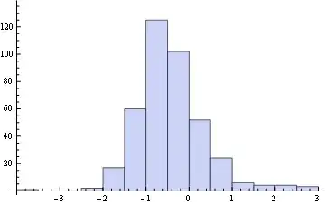
The problem is that the vector moduli spans many orders of magnitude so it can't be represented in a linear scale easily. See:

Histogram@Flatten@Map[Log[10, Norm@#] &, tr, {2}]

Now you have at least two alternatives. You may establish a cutoff and stop viewing "large" vectors to be able to represent the finer grain:

ListVectorPlot[tr, VectorScale -> {Automatic, Automatic, If[#5 > .5, 0, #5] &}]

Or you may represent the vectors' directions along with a background showing (for example) the Log of the modulus:

Show[
 ListDensityPlot[Map[Log@Norm@# &, tr, {2}],PlotLegends -> Automatic],
 ListStreamPlot@tr]

---

Edit

Note that if you give it some time Mathematica can cope with your functions without resorting to lists:

vecXY[A_?NumericQ, u_?NumericQ, v_?NumericQ, α_?NumericQ, ϕ_?NumericQ] := 
                           1/(16 π) Abs[Through[{ex, ez}[A, u, v, α, ϕ]]]^2

dp = DensityPlot[Log@Norm@vecXY[141.20, 0, Norm[{x, y}], Pi/2, ArcTan[x, y]], 
                 {x, 0, 20}, {y, 0, 20}, PlotLegends -> Automatic];
sp = StreamPlot[vecXY[141.20, 0, Norm[{x, y}], Pi/2, ArcTan[x, y]], 
                 {x, 0, 20}, {y, 0, 20}];

Show[dp, sp]