How to solve constraint differential equations using If function

Question

I have to solve a series of differential equations along with a constraint that has to be satisfied at each point of time where $t\in [0, 100]$ The model parameters are

β = 0.1; c1 = 10; c2 = 30; k1 = 100; k2 = 300; T = 100; 
δ1 = 0.1; δ2 = 0.3; Subscript[y, 0] = 1000; a = 4000; b = 200;

To solve the differential equations, I first assume that μ[t]=0solves the following in order to obtain $\lambda (t)$ and $x(t)$

sol1 = NDSolve[{λ'[t] == -((c1^2 - 4*k1*β*λ[t] - 
   2*c1*(λ[t] + μ[t]) + (λ[t] + μ[t])^2)/(
   4 k1)), x'[t] == -((c2^2 - 4*k2*(β*x[t] + δ1 (x[t] - λ[t])) - 2*c2*(x[t] + μ[t]) + 
   (x[t] + μ[t])^2)/(4 k2)), λ[T] == 0, x[T] == 0}, {λ, x}, {t, 0, 100}];

having λ[t] and x[t], I calculate ρ1[t] and ρ2[t]

ρ1[t_] := (c1 - {λ[t] /. sol1} - μ[t])/(2*k1);
ρ1[t][[1, 1]];

ρ2[t_] := (c2 - {x[t] /. sol1} - μ[t])/(2*k2);
ρ2[t][[1, 1]];

Having ρ1[t] and λ[t], ρ2[t] and x[t], I have to solve the following differential equations where `

d[t_] := a + b*Sin[(2*π*t/25)];

s = NDSolve[{y3'[t] == d[t] - δ2*y3[t], 
y2'[t] == δ2*y3[t] - (δ1 - ρ2[t][[1, 1]]) y2[t], 
y1'[t] == δ1*y2[t] - ρ1[t][[1, 1]]*y1[t], 
y3[0] == Subscript[y, 0], y2[0] == Subscript[y, 0], 
y1[0] == Subscript[y, 0]}, {y3, y2, y1}, {t, 0, 100}];

The problem is my constraint is based on ρ1[t], y1[t], ρ2[t] and y2[t]. So only after calculating everything with the assumption of μ[t]=0, I can actually check my constraint to see if it is satisfied, the constraint is the following: if

d[t] - (ρ1[t]*{y1[t] /. s} + ρ2[t]*{y2[t] /. s}) >= 0

then μ[t] = 0. Otherwise calculate the $μ[t]$ from below

μ[t] := (-2*d[t]*k1*k2 + c1*k2*{y1[t] /. s} + c2*k1*{y2[t] /. s} - 
 k2*{y1[t] /. s}*{λ[t] /. sol1} - 
 k1*{y2[t] /. s}*{x[t] /. sol1})/(k2*{y1[t] /. s} + 
 k1*{y2[t] /. s})]

and then I have to solve everything with from the beginning with new value of μ[t]. With μ=0 I get something like this

Plot[{d[t], ρ1[t]*{y1[t] /. s} + ρ2[t]*{y2[t] /. s}}, {t, 0,
   100}, PlotRange -> {0, 6000}, Frame -> True, 
 FrameLabel -> {"time", "d(t)-(ρ1(t)y1(t)+ρ2(t)y2(t))"}]

basically after the intersection point both lines should be adjusted (this should be taken care of by the new value of μ[t]) Is there anyways to code this model to check μ[t] at each point of time and see if the constraint is satisfied or not? do I need to create a loop to do this?

Answer 1

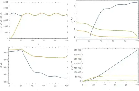
This interesting problem can be solved by iterating several times on μ. (WhenEvent cannot be used, because this is a boundary value, not an initial value, computation.)

μ[t_] = 0;
β = 1/10; c1 = 10; c2 = 30; k1 = 100; k2 = 300; T = 100; 
δ1 = 1/10; δ2 = 3/10; Subscript[y, 0] = 1000; a = 4000; b = 200;
d[t_] = a + b*Sin[(2*π*t/25)];
y3[t_] = DSolveValue[{y3t'[t] == d[t] - δ2*y3t[t], y3t[0] == Subscript[y, 0]},
    y3t[t], {t, 0, T}];

Do[sol1 = First@NDSolve[
    {λ'[t] == -((c1^2 - 4*k1*β*λ[t] - 2*c1*(λ[t] + μ[t]) + (λ[t] + μ[t])^2)/(4 k1)), 
     x'[t] == -((c2^2 - 4*k2*(β*x[t] + δ1 (x[t] - λ[t])) - 
         2*c2*(x[t] + μ[t]) + (x[t] + μ[t])^2)/(4 k2)),
     ρ1[t] == (c1 - λ[t] - μ[t])/(2*k1),
     ρ2[t] == (c2 - x[t] - μ[t])/(2*k2),
     λ[T] == 0, x[T] == 0}, {λ, x, ρ1, ρ2}, {t, 0, T}];
s = First@NDSolve[
     {y2'[t] == δ2*y3[t] - (δ1 - (ρ2[t] /. sol1)) y2[t], 
      y1'[t] == δ1*y2[t] - (ρ1[t] /. sol1)*y1[t], 
      y2[0] == Subscript[y, 0], y1[0] == Subscript[y, 0]}, {y2, y1}, {t, 0, T}];
μ[t_] = If[.99 d[t] >= ρ1[t]*y1[t] + ρ2[t]*y2[t], 0,
            Max[(-2*d[t]*k1*k2 + c1*k2*y1[t] + c2*k1*y2[t] - 
            k2*y1[t]*λ[t] - k1*y2[t]*x[t])/(k2*y1[t] + k1*y2[t]), 0]] /. s /. sol1, {i, 5}]

Grid[{{Plot[{d[t], (ρ1[t] /. sol1)*(y1[t] /. s) + (ρ2[t] /. sol1)*(y2[t] /. s)}, {t, 0, T},
         PlotRange -> {0, 6000}, Frame -> True, FrameLabel -> {"t", "d-(ρ1 y1 +ρ2 y2)"}, 
         ImageSize -> Medium],
      Plot[{μ[t], λ[t] /. sol1, x[t] /. sol1}, {t, 0, T}, Frame -> True, 
         FrameLabel -> {"t", "μ, λ, x"}, ImageSize -> Medium]},
     {Plot[{ρ1[t] /. sol1, ρ2[t] /. sol1}, {t, 0, T}, Frame -> True, 
         FrameLabel -> {"t", "ρ1, ρ2"}, ImageSize -> Medium],
      Plot[{y1[t] /. s, y2[t] /. s, y3[t]}, {t, 0, T}, Frame -> True, 
         FrameLabel -> {"t", "y1, y2, y3"}, ImageSize -> Medium]}}]

Several points are worth noting:

• The calculation of y3 is independent of μ and can be moved outside the iteration process. It is computed exactly here, although the gain in accuracy is negligible.
• ρ1 and ρ2 are calculated inside NDSolve, so that they are represented as single InterpolatingFunctions. Otherwise, FunctionInterpolation must be used, so that recursive definitions of μ do not accumulate in them, causing the iteration to fail.
• A safety factor is needed in the definition of μ so that the sign of the first argument of If does not oscillate during the iteration. However, this safety factor can allow μ to dip slightly negative near t = 21. Max is used to prevent this, even though its effect is negligible.
• Convergence is rapid, yielding no visible changes to the curves after four iterations.

Edit: Simplified expression for μ and corrected typo based on recommendations by MichaelE2.

Plotting Results for Several Parameter Values

As requested in a comment below, curves for several values of a parameter (here, δ1) can be computed and plotted as follows.

Do[δ1 = j/10; μ[t_] = 0; 
Do[sol1 = First@NDSolve[
    {λ'[t] == -((c1^2 - 4*k1*β*λ[t] - 2*c1*(λ[t] + μ[t]) + (λ[t] + μ[t])^2)/(4 k1)), 
     x'[t] == -((c2^2 - 4*k2*(β*x[t] + δ1 (x[t] - λ[t])) - 
         2*c2*(x[t] + μ[t]) + (x[t] + μ[t])^2)/(4 k2)),
     ρ1[t] == (c1 - λ[t] - μ[t])/(2*k1),
     ρ2[t] == (c2 - x[t] - μ[t])/(2*k2),
     λ[T] == 0, x[T] == 0}, {λ, x, ρ1, ρ2}, {t, 0, T}];
s = First@NDSolve[
     {y2'[t] == δ2*y3[t] - (δ1 - (ρ2[t] /. sol1)) y2[t], 
      y1'[t] == δ1*y2[t] - (ρ1[t] /. sol1)*y1[t], 
      y2[0] == Subscript[y, 0], y1[0] == Subscript[y, 0]}, {y2, y1}, {t, 0, T}];
μ[t_] = If[.99 d[t] >= ρ1[t]*y1[t] + ρ2[t]*y2[t], 0,
           Max[(-2*d[t]*k1*k2 + c1*k2*y1[t] + c2*k1*y2[t] - 
           k2*y1[t]*λ[t] - k1*y2[t]*x[t])/(k2*y1[t] + k1*y2[t]), 0]] /. s /. sol1, {i, 5}];
ρ1sav[j] = ρ1 /. sol1; ρ2sav[j] = ρ2 /. sol1, {j, 7}]

ParametricPlot3D[Evaluate[Table[{t, j, ρ1sav[j][t]}, {j, 7}]], {t, 0, T}, 
    PlotRange -> {Automatic, Automatic, {0, .05}}, BoxRatios -> {2, 1, .7}, 
    AxesLabel -> {"t", "10 δ1", "ρ1"}, LabelStyle -> Directive[Bold, 14], 
    ImageSize -> Large]

and similarly for ρ2. The plot design is based on the answer by Heike to question 1413.