28

Mathematica doesn't seem to have built-in tools to deal with the Eisenstein series:

$$\begin{align*} E_{2}(\tau)&= 1-24 \sum_{n=1}^{\infty} \frac{n e^{2 \pi i n \tau}}{1-e^{2 \pi i n \tau}}\\ E_{4}(\tau)&= 1+240 \sum_{n=1}^{\infty} \frac{n^{3} e^{2 \pi i n \tau}}{1-e^{2 \pi i n \tau}} \end{align*}$$

I'm wondering what is the best way to deal with this. Just messing around, informally, on Wolfram, it seems like these series all converge pretty fast. Can I carry out the sums manually in Mathematica including a small number of terms? Or is there a better way? I'm worried this is prone to severe inaccuracy for $\Im(\tau)$ either large or small, both cases I'm interested in.

If it simplifies anything, I only need the cases $\Re(\tau) \in \mathbb{Z}$ where the series outputs real numbers.

J. M.'s missing motivation
  • 124,525
  • 11
  • 401
  • 574
Benighted
  • 1,327
  • 1
  • 10
  • 14

3 Answers3

33

Since EllipticTheta[] is a built-in function, and since the Eisenstein series $E_4(q)$ and $E_6(q)$ are expressible in terms of theta functions (I use the nome $q$ as the argument in this answer, but you can convert to your convention by using the relation with the period ratio $\tau$: $q=\exp(2\pi i \tau)$), and since the higher-order Eisenstein series (note that they are only defined for even orders!) can be generated from $E_4(q)$ and $E_6(q)$ through a recurrence (see e.g. Apostol's book), it is relatively straightforward to write Mathematica routines for these functions:

SetAttributes[EisensteinE, {Listable, NHoldFirst}];

EisensteinE[4, q_] := (EllipticTheta[2, 0, q]^8 + EllipticTheta[3, 0, q]^8 +
                       EllipticTheta[4, 0, q]^8)/2

EisensteinE[6, q_] := With[{q2 = EllipticTheta[2, 0, q]^4,
                            q3 = EllipticTheta[3, 0, q]^4,
                            q4 = EllipticTheta[4, 0, q]^4}, 
                           (q2 + q3) (q3 + q4) (q4 - q2)/2

EisensteinE[n_Integer?EvenQ, q_] /; n > 2 := (6/((6 - n) (n^2 - 1) BernoulliB[n]))
Sum[Binomial[n, 2 k + 4] (2 k + 3) (n - 2 k - 5)
    BernoulliB[2 k + 4] BernoulliB[n - 2 k - 4]
    EisensteinE[2 k + 4, q] EisensteinE[n - 2 k - 4, q], {k, 0, n/2 - 4}]

Here are a few examples:

(* "equianharmonic case" *)
{ω1, ω3} = {1, (1 + I Sqrt[3])/2};
N[WeierstrassInvariants[{ω1, ω3}]] // Quiet // Chop
   {0, 12.825381829368068}

2 {60, 140} Zeta[{4, 6}] EisensteinE[{4, 6}, Exp[I π ω3/ω1]]/(2 ω1)^{4, 6}
// N // Chop
   {0, 12.825381829368068}

(* "lemniscatic case" *)
{ω1, ω3} = {1, I};
N[WeierstrassInvariants[{ω1, ω3}]] // Quiet // Chop
   {11.817045008077123, 0}

2 {60, 140} Zeta[{4, 6}] EisensteinE[{4, 6}, Exp[I π ω3/ω1]]/(2 ω1)^{4, 6}
// N // Chop
   {11.817045008077123, 0}

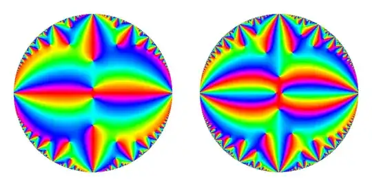
Using techniques similar to the one used in this answer, here are domain-colored plots of $E_4(q)$ (left) and $E_6(q)$ (right) over the unit disk, using the DLMF coloring scheme:

domain-colored plots of the Eisenstein series


Now, one may ask: what about $E_2(q)$? This function is what is termed as a "quasi-modular" form, whose behavior with respect to modular transformations is completely different from the other $E_{2k}(q)$. Due to this unusual state of affairs (i.e. not expressible entirely in terms of theta functions), one needs a different formula for $E_2(q)$; one useful formula can be found hidden deep within Abramowitz and Stegun:

EisensteinE[2, q_] := With[{q3 = EllipticTheta[3, 0, q]^2}, 6/π
                           EllipticE[InverseEllipticNomeQ[q]] q3 -
                           q3^2 - EllipticTheta[4, 0, q]^4]

Test:

Series[EisensteinE[2, q], {q, 0, 12}]
   1 - 24 q^2 - 72 q^4 - 96 q^6 - 168 q^8 - 144 q^10 - 288 q^12 + O[q]^13

1 - Sum[24 DivisorSigma[1, k] q^(2 k), {k, 1, 6}]
   1 - 24 q^2 - 72 q^4 - 96 q^6 - 168 q^8 - 144 q^10 - 288 q^12

Unfortunately, altho this version is great for symbolic use, it is not too good for numerical evaluation, as can be seen from the following attempt to generate a domain-colored plot from it:

wrong domain-colored plot of E2

The relatively complicated branch cut structure is apparently inherited from the branch cuts of the complete elliptic integral of the second kind $E(m)$ not being canceled out by the inverse nome.

Thus, I shall present another routine for numerically evaluating $E_2(q)$, based on recursing the quasi-modular relation (note the use of $\tau$ instead of $q$)

$$E_2\left(-\frac1{\tau}\right)=\tau^2 E_2(\tau)-\frac{6i\tau}{\pi}$$

before the actual numerical evaluation of the series:

e2[zz_ /; (InexactNumberQ[zz] && Im[zz] > 0)] :=
   Block[{τ = SetPrecision[zz, 1. Precision[zz]], r = False, f, k, pr, q, qp, s},
         τ -= Round[Re[τ]]; pr = Precision[τ];
         If[7 Im[τ] < 6,
            r = True; f = e2[SetPrecision[-1/τ, pr]],
            q = SetPrecision[Exp[2 π I τ], pr]; f = s = 0; qp = 1; 
            k = 0;
            While[k++; qp *= q; f = s + k qp/(1 - qp); s != f, s = f];
            f = 1 - 24 f];
         If[r, (f/τ + 6 I/π)/τ, f] /; NumberQ[f]]

EisensteinE[2, q_?InexactNumberQ] :=
   If[q == 0, N[1, Internal`PrecAccur[q]], e2[Log[q]/(I π)]]

(Note that the subroutine e2[] actually takes the period ratio $\tau$ as the argument; if your preferred convention is to use $\tau$ instead of $q$, you can make that the main routine and skip the conversion to $q$ altogether.)

This now gives a proper-looking plot:

domain-colored plot of E2

(Thanks to მამუკა ჯიბლაძე for convincing me to look further into this.)


Finally, if you prefer the function $G_{2k}(q)$, here is the corresponding formula:

EisensteinG[n_Integer?EvenQ, q_] := 2 Zeta[n] EisensteinE[n, q]
J. M.'s missing motivation
  • 124,525
  • 11
  • 401
  • 574
  • That's great :) +1 – Sektor Aug 01 '15 at 15:46
  • (+1) I have a degree in Chemical Engineering and my math courses seemed to have stopped way earlier than I realize! – kale Aug 01 '15 at 16:47
  • 7
    @kale, I am a chemist by trade, and I can confidently assure you that at least 80% of the mathematics I have ever used here, on math.SE, and MathOverflow, were definitely not taught in the classroom. ;) – J. M.'s missing motivation Aug 01 '15 at 17:00
  • @J.M. This is awesome, thank you :) I did notice in your examples, things seem to depend not just on $q$ alone but also $\omega_{1}$. Shouldn't this not be the case? Perhaps that can be absorbed into Zeta[{4,6}] – Benighted Aug 01 '15 at 17:10
  • 1
    @spietro, all the modular forms depend only on $\tau$, $q$, or any of a number of other possible arguments; in the case of the demonstration with the Weierstrass invariants, you must realize that they satisfy homogeneity relations, thus enabling the mathematician to concentrate entirely on $\tau$ and not have to carry around two complex numbers. – J. M.'s missing motivation Aug 01 '15 at 17:13
  • 1
    @J.M. +1. I didn't realize you are a chemist. Good to see fellow chemists here. – RunnyKine Aug 01 '15 at 20:30
  • Alternatively, for $E_2$, q D[Series[Log[DedekindEta[-((I Log[q])/(2 \[Pi]))]^24], {q, 0, 12}], q] gives the same series. In other words, $E_2$ is the logarithmic derivative of the modular discriminant. – მამუკა ჯიბლაძე Nov 14 '15 at 14:14
  • @მამუკა ჯიბლაძე, well, it's a truncation, yes... I'm still thinking if there's a neater implementation, tho. – J. M.'s missing motivation Nov 14 '15 at 14:34
  • 1
    In fact $e^{2\pi i\tau}\frac d{dq}\log\eta(\tau)$ (with $q=e^{2\pi i\tau}$) does not seem to have any branch cuts, and only coincides with yours near the origin – მამუკა ჯიბლაძე Nov 14 '15 at 16:50
  • @J.M. I keep coming back to your wonderful answer to my question here! You mention that $E_2$ has a complicated branch cut structure...do you recall anywhere this is discussed? I can't seem to find anything. – Benighted May 06 '16 at 22:06
  • 1
    @spietro, I've fixed the routine for $E_2$, if you're still interested in this. – J. M.'s missing motivation Jan 08 '17 at 05:35
  • I am now going to switch sides :D - honestly speaking I still cannot explain why exactly were these cuts avoidable. If there is a branch without any ambiguities, how could they appear in the first place?? Besides, $E_2$ must have some problems, it is well known that it is not fully modular, as evident from the functional equation you displayed above. So in principle it should not be possible to descend from $\tau$ to $q$ unambiguously... – მამუკა ჯიბლაძე Jan 08 '17 at 08:28
  • 1
    @მამუკა ჯიბლაძე, "If there is a branch without any ambiguities, how could they appear in the first place?" - that's a good question. I was satisfied when taking the long route via WeierstrassZeta[] was providing consistent results with the routine. Currently, the only thing that could contribute possible branch cuts in the $q$-version would be the logarithm; is there any other possible branch cut choice that would give "reasonable" (whatever that means here) results? – J. M.'s missing motivation Jan 08 '17 at 09:08
  • Well there might be several obstructions to univaluedness - one possibility you mentioned yourself in the answer, elliptic integrals are similar to the logarithm in this respect. Another is the one I mentioned, ambiguities inherent in the functional equation. Also, the series for $E_2$ does not converge absolutely, so rearranging terms might give different results. Unfortunately I don't know enough to sort all this out. But I feel there is something very important hidden behind all this. – მამუკა ჯიბლაძე Jan 08 '17 at 09:34
  • 1
    In fact current point of view (see e. g. 2.3 (page 19) of Zagier's notes) is that $E_2$ is the holomorphic part of the nonholomorphic modular form $E_2^*(z):=E_2(z)-\frac3{\pi\operatorname{Im}(z)}$, so maybe the unambiguous version of your plot can be explained by that, I don't know. – მამუკა ჯიბლაძე Jan 08 '17 at 09:36
  • Thanks for the great answer @J.M.. Is there a way to do a similar plot for the 'magnitude' or 'real part' or 'imaginary part' of Eisenstein series instead of the 'Arg'? I used the code from https://mathematica.stackexchange.com/a/89673 and replaced the Arg by Re, and changed the ColorFunction appropriately but I do not get a proper plots. Ideally, I would have liked to reproduce something along the lines of the disc plots for $G_6$ as on the Wikipedia page (https://en.wikipedia.org/wiki/Eisenstein_series) – TheTwistedSector Jul 12 '20 at 15:44
  • @The, it should be possible, but I think you should ask that as a separate question. – J. M.'s missing motivation Aug 04 '20 at 01:24
  • 3
    Just an update: the code of this answer here was used in generating some plots in this paper: https://arxiv.org/pdf/2007.10998.pdf. This webpage has been cited as ref [63]. I am, once gain, very grateful to @J.M. for this amazing answer. – TheTwistedSector Feb 15 '21 at 04:46
6

The above expression for EisensteinE[2, q] is a bit slow. Here is a faster version using double precision arithmetic:

EisensteinE[2, tau_Complex /; Im[tau] > 0] := ee2Upper[tau];
ee2Upper = Compile[
    {{tauIn, _Complex}},
    Block[{tau = tauIn, f, k, q, qp, s},
         tau -= Round[Re[tau]];
         If[7 Im[tau] < 6,
            f = ee2Upper[-1/tau]; (f/tau + 6 I/Pi)/tau,
            q = Exp[2 Pi I tau]; f = s = 0.0 + 0.0 I; qp = 1.0 + 0.0 I; 
            k = 0;
            While[k++; qp *= q; f = s + k qp/(1 - qp);
                  Abs[s - f] > MachinePrecision, s = f];
            1 - 24 f]],
    {{ee2Upper[_], _Complex}}];

Note that it is expressed in terms of τ instead of q.

5

Since 11.2 (2017) Mathematica does have the built-in tools to deal with the Eisenstein series:

$$G_{2k}(\tau)=\sum_{(m,n)}{'}\frac{1}{(m+n \tau)^{2k}}$$ being the functions:

WeierstrassInvariantG2
WeierstrassInvariantG3

Calculating $G_{2k}(\tau)$ can be implemented as follows:

g2[2, t_] = WeierstrassInvariantG2[{1/2, t/2}]/60;
g2[3, t_] = WeierstrassInvariantG3[{1/2, t/2}]/140;
g2[m_, t_] :=  3 Sum[(2 r - 1) (2 m - 2 r - 1) g2[r, t] g2[m - r, t], {r, 2, m - 2}]/((2 m + 1) (m - 3) (2 m - 1))

( Updated 17/6-'21 ):

nEisensteinG2K[2, t_]=nEisensteinG2K[2, {1, t}];
nEisensteinG2K[3, t_]=nEisensteinG2K[3, {1, t}];
nEisensteinG2K[2, {w1_, w3_}]=WeierstrassInvariantG2[{w1/2,w3/2}]/60;
nEisensteinG2K[3, {w1_, w3_}]=WeierstrassInvariantG3[{w1/2,w3/2}]/140;
nEisensteinG2K[m_, {w1_, w3_}]:= 3 Sum[(2 r - 1) (2 m - 2 r - 1) nEisensteinG2K[r, {w1, w3}] nEisensteinG2K[m - r, {w1, w3}], {r, 2, m - 2}]/((2 m + 1) (m - 3) (2 m - 1))

Source/Reference:

Modular Functions and Dirichlet Series in Number Theory, Tom Apostol ( Chapter 1 Par 1.9 "The Eisenstein series and the invariants g2 and g3" )

nilo de roock
  • 9,657
  • 3
  • 35
  • 77