How do I split up a curve into chords of equal length?

Question

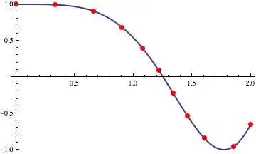
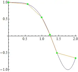
I have a curve that is defined as f[x] and what I'm attempting to do is to divide the curve into equal straight lengths for a number of segments of my choosing that I've defined as nSeg.

I've created a sheet that can work through and determine the (x,y) co-ordinates for each segment, but I'm having to manually manipulate the equations to create a single equation for Mathematica to find the roots for.

The straight length of the curve I've defined as;

chordL = Table[
            Sqrt[(Subscript[x, i + 1] - Subscript[x,i])^2 + 
                 (f[Subscript[x, i + 1]] - f[Subscript[x, i]])^2
            ], {i, 1, nSeg}
         ]

This creates a list of equations for the length of each segment. What I would like to do is make each part of the list equal to each other so that I can feed this into FindRoot later in the sheet so that if I decide to change the number of segments from 8 to 10, the sheet can be refreshed from a single variable.

FindRoot[*combined equations*, {Subscript[x, 2], 1}, {Subscript[x, 3], 2}]

The above is an example of how I'm currently doing it and it means I've a sheet for each value of nSeg, which isn't a smart way to work and I'm manually defining which variables to solve independently of the value of nSeg, even though the first and last co-ordinate will always be known.

I'm quite new to Mathematica and would really appreciate a nudge in the right direction to combine the equations in the first part to give the equations to solve in FindRoot (which I'm using instead of Solve for speed) in a flexible manner, and also increment the number of variables to solve given that x1 will always be 0 and x(nSeg+1) will always be known too as these are the start and end points of the curve which are defined by the input at the beginning of the sheet.

Answer 1

Straight segments

I'll assume you want to fix the first and last point and then plot the segments. Quick and dirty approach (I'll fix the first point at $x=0$ and the last at x=upVal; also note that actually nSeg isn't the number of segments here, but never mind):

upVal = 6;
nSeg = 10;
chordL = Table[
   Sqrt[(x[i + 1] - x[i])^2 + (f[x[i + 1]] - f[x[i]])^2], {i, 1, 
    nSeg}];
combEqs = # == d & /@ chordL;

That is, I set the length of all the segments to $d$, for which I will solve. Here's how to define the list of vars (with initial conditions, which are arbitrarily chosen here):

ClearAll[vars, x];
vars = Append[{x[#], #, x[1]+10^-6, upVal-10^-6} & /@ Range[2, nSeg],{d, 1}]

you can see I am adding $d$, the segment length, as a variable to solve for. Let's try for $f(x)=\sin(x)$:

f[x_] := Sin[x];
x[1] = 0;
x[nSeg + 1] = upVal;
sol = FindRoot[combEqs, vars];


points = Table[{{x[i], f[x[i]]}, {x[i + 1], f[x[i + 1]]}}, {i, 1, 
    nSeg}];

Show[
 Plot[f[x], {x, x[1], 1.1 x[nSeg + 1]}],
 Graphics@Line[points /. sol],
 Graphics[{Red, PointSize[Large], Point[Flatten[points, 1] /. sol]}]
 ]

So it seems to work.

Curved segments

If I just want to split up the curve in segments of equal length along the curve, I could do it like this:

ClearAll[findx, length];
findx[ell_, f_] := x /. FindRoot[length[x, f] \[Equal] ell, {x, 1}]
length[xf_?NumericQ, f_] := NIntegrate[Sqrt[1 + f'[z]^2], {z, 0, xf}]

Here, length gives the length of a curve f[x] from x=0 to x=xf, and findx uses that to obtain the coordinate x at which the length from x=0 to x=xf is ell. Then, we find the total length, split it into equal pieces $\delta L$, and use findx to obtain the values $x_n$ at which the length from the starting point is $n\delta L$:

nsegs = 10;
f[x_] := Cos[x^2]
xup = 2;
totalLength = length[xup, f];
dL = totalLength/nsegs;
xvals = Table[findx[n*dL, f], {n, 0, nsegs}];
Show[
 Plot[f[x], {x, 0, xup}],
 Graphics[{Red, PointSize[Large], 
   Point[Transpose[{xvals, f /@ xvals}]]}]
 ]

And here is the result:

Well, unless I messed it up.

Answer 2

I present here a variation of acl's approach for finding points along a curve with equal Euclidean distances. The most noticeable difference is that this version takes the optimization route, via NArgMax[]:

segmentCurve[ff_?VectorQ, {t_, tmin_, tmax_}, n_, opts___] := Block[{c, lens, vars},
             vars = c /@ Range[n - 1];
             lens = SquaredEuclideanDistance @@@
                    Partition[Function[t, ff] /@ Flatten[{tmin, vars, tmax}], 2, 1];
             NArgMax[{Total[lens], Equal @@ lens, Less @@ Flatten[{tmin, vars, tmax}]},
                     vars, opts]]

I have written the routine so that it takes a parametrically represented curve as input, thus allowing it to be used for both plane and space curves.

Here's how you might split a function curve like $\cos(x^2)$ into five segments:

vals = segmentCurve[{x, Cos[x^2]}, {x, 0, 2}, 5, WorkingPrecision -> 20]
  {0.57191013658298125958, 0.99139112961697439451,
   1.2387523086033325871, 1.4468296680931848997}

Build the corresponding points:

pts = Function[x, {x, Cos[x^2]}] /@ Flatten[{0, vals, 2}];

Check that they're equidistant:

Differences[EuclideanDistance @@@ Partition[pts, 2, 1]] // Chop
  {0, 0, 0, 0}

Show the points:

Plot[Cos[x^2], {x, 0, 2}, AspectRatio -> 1,
     Epilog -> {{Orange, Line[pts]},
                {Directive[AbsolutePointSize[6], Green], Point[pts]}}]

Here's how to apply the function to a space curve:

vals = segmentCurve[{Cos[t], Sin[t], t}, {t, 0, 2 π}, 8];
pts = Function[t, {Cos[t], Sin[t], t}] /@ Flatten[{0, vals, 2 π}];
Show[ParametricPlot3D[{Cos[t], Sin[t], t}, {t, 0, 2 π}], 
     Graphics3D[{{Orange, Line[pts]},
                 {Directive[AbsolutePointSize[6], Green], Point[pts]}}]]