Sparse Hessian for FindMinimum? Broken?

Question

Is the sparse Hessian mechanism for FindMinimum[] (Method->"Newton") broken? Or am I simply not apprehending its proper setup? Here's what's happening.

Below is for solving the example problem given in tutorial/UnconstrainedOptimizationNewtonsMethodMinimum#509267359
using specified Gradient g and (dense) Hessian h functions.

The only difference here from the documentation example is I specify g and h as bare symbolic expressions using RuleDelayed rather than as functions with x_?NumberQ type arguments. Nonetheless, the correct result is obtained:

Clear[f, g, h, x, y]
f = Cos[x^2 - 3 y] + Sin[x^2 + y^2]    
g = D[f, {{x, y}}]

(* Out[3]= {2 x Cos[x^2 + y^2] - 2 x Sin[x^2 - 3 y], 2 y Cos[x^2 + y^2]  + 3 Sin[x^2 - 3 y]}  *)

h = D[f, {{x, y}, 2}]    
(* Out[4]= {{-4 x^2 Cos[x^2 - 3 y] + 2 Cos[x^2 + y^2] - 
2 Sin[x^2 - 3 y] - 4 x^2 Sin[x^2 + y^2], 
6 x Cos[x^2 - 3 y] - 4 x y Sin[x^2 + y^2]}, 
{6 x Cos[x^2 - 3 y] - 4 x y Sin[x^2 + y^2],
-9 Cos[x^2 - 3 y] + 2 Cos[x^2 + y^2] - 4 y^2 Sin[x^2 + y^2]}} *)

FindMinimum[f, {{x, 1}, {y, 1}}, Method -> {"Newton", 
"Hessian" :> {h, "EvaluationMonitor" :>  Print[h]}}, 
Gradient :> {g, "EvaluationMonitor" :>  Print[g]}]

(* Output: 
{0.986301,-3.56019}
{{-0.986301,-6.13407},{-6.13407,-0.724162}}
{-0.527482,2.63714}
{{12.3165,2.2687},{2.2687,20.8245}}
{0.230844,-0.059627}
{{15.6441,0.981772},{0.981772,20.2644}}
{0.00357296,0.0000289779}
{{15.1633,0.983822},{0.983822,20.2729}}
{9.20305*10^-7,7.95904*10^-9}
{{15.1555,0.983708},{0.983708,20.2718}}
{5.85103*10^-14,2.82458*10^-15}
{{15.1555,0.983708},{0.983708,20.2718}}}
Out[5]= {-2., {x -> 1.37638, y -> 1.67868}}  *)

Now onto replicating the above, but this time specifying a sparse Hessian. I attempt to follow the setup discussed in:
tutorial/UnconstrainedOptimizationSpecifyingDerivatives#562305099

We first obtain the sparse Hessian function (sparhess), per the cells below:
1. convert the dense 2D list-based Hessian into a SparseArray form,
2. perform the indepotent Transpose[Transpose to force consistent lexicographic array index ordering of the non-zero element Rules
3. obtain those ArrayRules to form our sparse Hessian function, which is a same-ordered 1D list of the non-zero element functions...
4. ... parsing out the RHS expression of each Rule, and omitting the last ArrayRule, which is the default value for "zero" elements:

sphess = SparseArray[h];
sparsity = Transpose[Transpose[sphess]];
arhess = ArrayRules[sparsity]    
(* Out[8]={{1, 1} -> -4 x^2 Cos[x^2 - 3 y] + 2 Cos[x^2 + y^2] - 
2 Sin[x^2 - 3 y] - 4 x^2 Sin[x^2 + y^2], 
{1, 2} -> 6 x Cos[x^2 - 3 y] - 4 x y Sin[x^2 + y^2], 
{2, 1} -> 6 x Cos[x^2 - 3 y] - 4 x y Sin[x^2 + y^2],
{2, 2} -> -9 Cos[x^2 - 3 y] + 2 Cos[x^2 + y^2] - 4 y^2 Sin[x^2 + y^2], 
{_, _} -> 0}  *)

sparhess = arhess[[1 ;; -2, 2]]
(* Out[9]= {-4 x^2 Cos[x^2 - 3 y] + 2 Cos[x^2 + y^2] - 
2 Sin[x^2 - 3 y] - 4 x^2 Sin[x^2 + y^2], 
6 x Cos[x^2 - 3 y] - 4 x y Sin[x^2 + y^2], 
6 x Cos[x^2 - 3 y] - 4 x y Sin[x^2 + y^2],
-9 Cos[x^2 - 3 y] + 2 Cos[x^2 + y^2] - 4 y^2 Sin[x^2 + y^2]}

Next, we obtain the "SparseArray template" (sparsity) which specifies the sparsity pattern (non-zero elements) of the Hessian, per the cells below:
1. Take our earlier ArrayRules (arhess) and replace the RHS of Rules with Pattern "_", omitting the last ArrayRule, which is the default value for "zero" elements
2. Form a SparseArray from these ArrayRules
3. To be safe, do the trick to force consistent internal ArrayRule ordering:

arhess = Map[ReplacePart[#, 2 -> _] &, arhess[[1 ;; -2]]]
(* Out[10]= {{1, 1} -> _, {1, 2} -> _, {2, 1} -> _, {2, 2} -> _} *)
sparsity = SparseArray[arhess];
sparsity = Transpose[Transpose[sparsity]];

Now finally onto employing this in FindMinimum:

FindMinimum[f, {{x, 1}, {y, 1}}, Method -> {"Newton", 
"Hessian" :>  {sparhess, "Sparse" -> sparsity, 
"EvaluationMonitor" :>  Print[sparhess]}}, 
Gradient :> {g, "EvaluationMonitor" :>  Print[g]}]

(* Output: 
{0.986301,-3.56019}
{-0.986301,-6.13407,-6.13407,-0.724162}
{-9.46857,-4.5823}
{-13.6137,-3.30307}
{0.0908205,0.636614}
{1.36673,-0.619934,-0.619934,6.60192} 
{-0.111213,-0.102242}
{2.29398,0.384308,0.384308,7.15042}
{-0.00442004,-0.00834982}
{2.19695,0.0162966,0.0162966,7.16648}
{-0.0000188381,-0.0000167613}
{2.18754,0.000069903,0.000069903,7.16556}
{-1.63506*10^-10,-3.03399*10^-10}
{2.18752,6.06735*10^-10,6.06735*10^-10,7.16555}
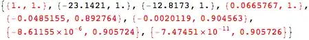
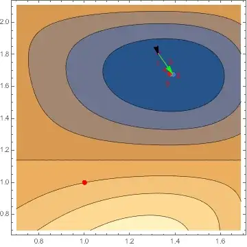
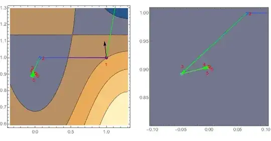
Out[13]= {-0.179902, {x -> -7.47451*10^-11, y -> 0.905726}}  *)

Wrong Answer! Comparing the gradient and hessian values printout for this FindMinimum run to the earlier correct run, we see that the first gradient and Hessian values are identical, but then our sparse version goes off the rails.

Interestingly, rerunning the above as so, using our original dense Hessian h to drive the minimization, setting "Sparse" to False, but along the minimization path printing out the values of sparhess, we observe the correct values being computed from sparhess (!?):

FindMinimum[f, {{x, 1}, {y, 1}}, Method -> {"Newton", 
"Hessian" :>  {h, "Sparse" -> False, 
"EvaluationMonitor" :>  Print[sparhess]}}, 
Gradient :> {g, "EvaluationMonitor" :>  Print[g]}]

(* Output: 
{0.986301,-3.56019}
{-0.986301,-6.13407,-6.13407,-0.724162}
{-0.527482,2.63714}
{12.3165,2.2687,2.2687,20.8245}
{0.230844,-0.059627}
{15.6441,0.981772,0.981772,20.2644}
{0.00357296,0.0000289779}
{15.1633,0.983822,0.983822,20.2729}
{9.20305*10^-7,7.95904*10^-9}
{15.1555,0.983708,0.983708,20.2718}
{5.85103*10^-14,2.82458*10^-15}
{15.1555,0.983708,0.983708,20.2718}
Out[14]= {-2., {x -> 1.37638, y -> 1.67868}}  *)

Answer 1

I can't be sure what FindMinimum does. I can only find the various *Monitor options to see what major steps it takes. Then I might only infer, rightly or wrongly, why it does any of these things. I will say that I think it is behaving "correctly" in the sense of "as intended."

When all the conditions are "right," the step taken by FindMinimum under Newton's method is given by

LinearSolve[h, -g, Method -> {"Cholesky", "Modification" -> "Minimal"}]

where h denotes the Hessian and g the gradient of f. The Hessian matrix h needs to be "sufficiently positive definite" for CholeskyDecomposition. But LinearSolve returns an answer whether or not h is positive definite, and sometimes FindMinimum accepts it when h is not. I also suspect that this is only an approximate description of what happens. For instance, there are internal functions that might be used:

One thought is that sparse systems, which typically have a large number of variables, exhibit certain issues in general, and FindMinimum might be applying a different strategy than on a small dense system. It may also automatically apply sparse methods to sparse input that is neither large nor sparse.

It does seem that the OP has set up the sparse Hessian correctly, and it works as expected in a basin in which the Hessian is positive definite (which is typical of local minima, except in pathological cases).

Analysis of the example

(See below for auxiliary functions fmdata, which gathers data about the steps FindMinimum takes and fmdataplot which plots it.)

Below are the steps FindMinimum takes on the basic example. The black arrow indicates the direction of the gradient at the initial point, and the green arrow is the step at the initial point predicted by LinearSolve. In this case it is the step FindMinimum takes.

fm0 = fmdata@ FindMinimum[f, {{x, 1}, {y, 1}}, 
    Method -> {"Newton", "Hessian" :> h}, Gradient :> g];
plot = fmdataplot[fm0]

Below is the same plot for the sparse method. Note the step by LinearSolve would be identical, but FindMinimum ignores it (as though it did not even bother to compute it).

fmsp = fmdata@ FindMinimum[f, {{x, 1}, {y, 1}}, 
    Method -> {"Newton", "Hessian" :> {sparhess, "Sparse" -> sparsity}}, Gradient :> g];
fmdataplot[fmsp]

What has happened is that FindMinimum went far to the left and searched back toward the initial point, apparently looking for a point where the Hessian is positive definite. This can be seen in the points that are evaluated (the points in red are the initial point plus the actual steps; the black pairs are extra evaluations done to determine the next step):

fmsp["eval"] /. (# -> Style[#, Red] & /@ fmsp["steps"])

If we manually apply the LinearSolve step first, the sparse method follows the default method, probably because the step lands in a basin where the Hessian is positive definite.

fmsp1 = Module[{x0, y0},
   {x0, y0} = {1., 1.} + 
     LinearSolve[
      h /. Thread[{x, y} -> {1., 1.}], -g /. Thread[{x, y} -> {1., 1.}], 
      Method -> {"Cholesky", "Modification" -> "Minimal"}];
   fmdata@
    FindMinimum[f, {{x, x0}, {y, y0}}, 
     Method -> {"Newton", "Hessian" :> {sparhess, "Sparse" -> sparsity}}, Gradient :> g]
   ];
Show[fmdataplot[fmsp1], 
  Graphics[{Red, PointSize[Large], Point[{1, 1}]}], 
  PlotRange -> PlotRange[plot]] /. 
 gc_GraphicsComplex :> Cases[plot, _GraphicsComplex, Infinity]

Code dump

Aside from fmdata and fmdataplot used above, I include two more

• fmLSsteps, which computes the steps predicted by LinearSolve, which can be compared with the actual steps taken by FindMinimum.
• fmLSstepgraphics, which creates an arrow for each step representing the predicted step.

The data structure returned by fmdata is an Association with the following keys:

• "result": The result of FindMinimum
• "eval": The points where the function was evaluated (from EvaluationMonitor)
• "steps": The steps taken (points, from StepMonitor)
• "variables": The variables passed to FindMinimum
• "initialpoint": The initial point passed to FindMinimum
• "function": The function passed to FindMinimum
• "gradient": The gradient used (computed with D)
• "hessian": The Hessian used (computed with D)
• "method": The Method option passed to FindMinimum

The function fmdataplot is used instead of Optimization`UnconstrainedProblems`FindMinimumPlot because FindMinimumPlot did not work with the sparse method. It would never finish. There is an optional second argument

fmdataplot[data, points]

where points can be either "steps" or "eval"; it determines whether to plot the steps or the evaluation points. The default is "steps".

ClearAll[fmdata, fmdataplot, fmLSsteps, fmLSstepgraphics];
SetAttributes[fmdata, HoldAll];
fmdata[FindMinimum[obj_, init_List, opts : OptionsPattern[FindMinimum]]] := 
  Module[{f, g, h, var, var0, min, ptsS, ptsE},
   f = First@Flatten[{obj}];
   var = init[[All, 1]];
   var0 = N@init[[All, 2]];
   g = D[f, {var}];
   h = D[f, {var, 2}];
   {min, {{ptsS}, {ptsE}}} = Reap[
     Sow[var0, "step"]; (* add step 0 *)
     FindMinimum[obj, init,
      StepMonitor :> Sow[var, "step"], 
      EvaluationMonitor :> Sow[var, "eval"],
      opts
      ],
     {"step", "eval"}
     ];
   <|"result" -> min, "eval" -> ptsE, "steps" -> ptsS, 
    "variables" -> var, "initialpoint" -> var0, "function" -> f, 
    "gradient" -> g, "hessian" -> h, 
    "method" -> OptionValue[FindMinimum, {opts}, Method]|>];
fmdataplot[data_, pts_: "steps"] := 
 With[{p0 = data@"initialpoint", 
    eval = Thread[data@"variables" -> data@"initialpoint"]},
  MinMax /@ Transpose[data[pts]] /. {{x1_, x2_}, {y1_, y2_}} :>
    Show[
     ContourPlot[data["function"], {x, x1 - 0.3, x2 + 0.3}, {y, y1 - 0.3, y2 + 0.3}],
     Graphics[{{PointSize[Large], Thick,
          Line[#, VertexColors -> ColorData[{"Rainbow",{1,Length@#}}] /@ Range[Length@#]],              
          Point[#,VertexColors -> ColorData[{"Rainbow",{1,Length@#}}] /@ Range[Length@#]],
          Red, 
          MapIndexed[
           Text[First@#2, #1, 
             2.5 {Cos[1.5 First@#2], Sin[1.5 First@#2]}] &, #]} &[
        data@pts],
       Tooltip[
        Arrow[{p0, 
          p0 - 0.1 Sqrt[(x1 - x2)^2 + (y1 - y2)^2]*Normalize@data@"gradient" /. eval}],
        "gradient"],
       Green, 
       Tooltip[Arrow[{p0, 
          p0 + LinearSolve[data@"hessian" /. eval, -data@"gradient" /. eval, 
            Method -> {"Cholesky", "Modification" -> "Minimal"}]}], 
        "LS step"]}]
     ]
  ]
fmLSsteps[data_, pts_: "steps"] := LinearSolve[
     data@"hessian" /. Thread[data@"variables" -> #],
     -data@"gradient" /. Thread[data@"variables" -> #], 
     Method -> {"Cholesky", "Modification" -> "Minimal"}] & /@ 
   data[pts];
fmLSstepgraphics[data_, pts_: "steps"] := MapThread[
  Tooltip[Arrow[{#, # + #2}], "LS step"] &,
  {data@pts, fmLSsteps[data, pts]}]

Example of fmLSstepgraphics: The sparse method steps, with close-up (right). One can see the first step is different, but inside the basin, the steps agree.

GraphicsRow[{
  foo = Show[fmdataplot[fmsp], 
    Graphics[{Green, fmLSstepgraphics[fmsp]}]],
  Show[foo, PlotRange -> ({-0.1, 0.1} + # & /@ fmsp["result"][[2, All, 2]])]
  }]