How to find roots of equation

Question

Solve[(Cos[θ] - Cos[θi]) + (θ - θi)*Sin[θi] == 0, θ]

Hi, I am new to Mathematica, and I am trying to find roots of the above equation, but not success.

Answer 1

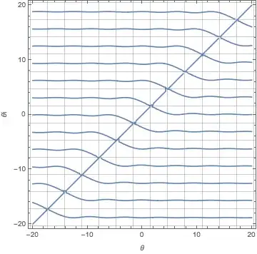
A plot of the equation, which is a form of a numerical solution, is highly suggestive that this is not a "random" equation and might have some structure:

eqn = (Cos[θ] - Cos[θi]) + (θ - θi) Sin[θi] == 0;

cplot = ContourPlot[Evaluate@eqn,
 {θ, -20, 20}, {θi, -20, 20},
 FrameLabel -> Automatic,
 GridLines -> {Range[Pi/2 - 7 Pi, 7 Pi, Pi], Range[Pi/2 - 7 Pi, 7 Pi, Pi]}]

Let's replace θi by θ + u and see if we can tease out a factor of u. Terms in Sin[u] can have a u factored out thus:

Sin[u] -> u Sinc[u]

And factors of the form 1 - Cos[u] can have u factored via this transformation:

Cos[u] -> 1 - (u^2 Sinc[u]^2)/(1 + Cos[u])

We can then factor the function and throw away any factors that do no contain θ with FactorList; factors with a θ can be selected with the criterion ! FreeQ[#, θ] &.

The intermediate steps are irrelevant, so I'll use % in the code below (be sure $HistoryLength is positive).

(Cos[θ] - Cos[θi]) + (θ - θi) Sin[θi] /. θi -> θ + u // TrigExpand;
% /. {Sin[u] -> u Sinc[u], Cos[u] -> 1 - (u^2 Sinc[u]^2)/(1 + Cos[u])};
Select[FactorList@%, ! FreeQ[#, θ] &]
neweqn = %[[1, 1]];
(*  FactorList output -->
 {{-Sin[θ] - Cos[u] Sin[θ] - u Cos[θ] Sinc[u] - u Cos[u] Cos[θ] Sinc[u] +
   Sin[θ] Sinc[u] + Cos[u] Sin[θ] Sinc[u] + u Cos[θ] Sinc[u]^2 + u^2 Sin[θ] Sinc[u]^2, 1}}
*)

Now this can be solved:

sol = Solve[neweqn == 0, θ]

Short form:

There are two solutions. Each gives {θ, θi} == {θ, θ + u} in terms of u and ArcTan, which has a branch cut. On a whim, I thought, "Maybe we can integrate the branch cut." I'm glad I did, because while the prime motivation was wishful thinking, the solution became a whole lot simpler.

dθ = D[Simplify[θ /. First[sol], C[1] == 0], u];
Integrate[dθ, {u, 0, t}]
(*  -(1/2) (1 + π Sqrt[1/t^2]) t + ArcTan[t/(2 - t Cot[t/2])]  *)

It still has an ArcTan. We get the same result using the other solution Last[sol]. Solving for an appropriate initial condition, we get a parametrization for θ:

res = θ -> -(1/2) t + ArcTan[t/(2 - t Cot[t/2])]

The branch jumps, reflected in the diagonal red lines, should actually be discontinuities. Apparently they need to be excluded explicitly in ParametricPlot. Translating the solution res by multiples of Pi yields all solutions, except the trivial one θ == θ1 (corresponding to the factor u we took out).

Show[cplot, 
 ParametricPlot[{θ, θ + t} /. res, {t, -35, 35}, PlotStyle -> Red]]

Show[cplot,
 ParametricPlot[
  Evaluate@Table[Pi n + {θ, θ + t} /. res, {n, -5, 5}],
  {t, -35.001, 35}, Exclusions -> (2 - t Cot[t/2]) t == 0]]

Maybe more can be done, but that's what I got right now.

Answer 2

You can plot your equation as a function of θ for a given θi. You can also find the roots.

In the expressions below I have replaced the symbol θ with x as I was unable to paste it without it showing up as [Theta].

Below Manipulate is used to select the value of xi that will be plotted. There are also Manipulate parameters for setting the starting value for the two roots.

Manipulate[
 Column[{
   solBig = 
    FindRoot[(Cos[x] - Cos[xi]) + (x - xi)*Sin[xi] == 0, {x, xbig}],
   solSmall = 
    FindRoot[(Cos[x] - Cos[xi]) + (x - xi)*Sin[xi] == 0, {x, xsmall}],

   Show[
    Plot[(Cos[x] - Cos[xi]) + (x - xi)*Sin[xi], {x, -4 π, 4 π},
     PlotRange -> {{-4 π, 4 π}, {-5, 5}},
     PlotStyle -> Black,
     ImageSize -> 400
     ],
    ListPlot[{{x, 0}} /. solBig, 
     PlotStyle -> Directive[PointSize[Large], Red]],
    ListPlot[{{x, 0}} /. solSmall, 
     PlotStyle -> Directive[PointSize[Large], Blue]]
    ]

   }],

 {{xi, -3.}, -4 π, 4 π, Appearance -> "Open"},
 {{xbig, 2.}, -10, 10, Appearance -> "Open"},
 {{xsmall, -2.}, -10, 10, Appearance -> "Open"}
 ]

Below is an example with xi set to $-3.$ The two solutions (blue and red dots) are $-3.$ and $1.87728$.

Answer 3

Polynomials + trig generally don't mix. See this blog post on transcendental equations.

Your best bet would be to solve over the Reals and pick a numerical value for θi.

With[{θi = π/4},
  Solve[(Cos[θ] - Cos[θi]) + (θ - θi)Sin[θi] == 0, θ, Reals]
]

{{θ -> π/4}, {θ -> π/4}, 
 {θ -> Root[{4 Sqrt[2] + Sqrt[2] π - 8 Cos[#1] - 4 Sqrt[2] #1 &, 3.19740930731097365214214291155}]}}

Answer 4

If " i " represents the imaginary unit then:

eq = (Cos[θ] - Cos[θ I]) + (θ - θ I)*
Sin[θ I] == 0;
sol = FindRoot[eq, {θ, 5 + 5 I}]

$\{\theta \to 2.68471\, +4.77788 i\}$

These equation has infinite solutions:

sol2 = Chop@
Table[FindRoot[eq, {θ, n + m I}, 
WorkingPrecision -> 20], {n, -10, 10}, {m, -10, 10}] // Column