How can I fix a defect in the 3D graphics rendering of a coiled tube?

Question

I use the following code to obtain a tube version of a spring:

 p = 
   ParametricPlot3D[
     {20 Cos[t]-((837+800 Cos[2 t]-35 Cos[12 t]+40 Sqrt[2] Cos[t] Sqrt[801+Cos[12 t]]) Cos[300 t]+480 Sin[t] Sin[6 t] Sin[300 t])/(-1637+35 Cos[12 t]-40 Sqrt[2] Cos[t] Sqrt[801+Cos[12 t]]),
      20 Sin[t]+(4 (40 Cos[t]+Sqrt[2] Sqrt[801+Cos[12 t]]) (10 Cos[300 t] Sin[t]-3 Sin[6 t] Sin[300 t]))/(1637-35 Cos[12 t]+40 Sqrt[2] Cos[t] Sqrt[801+Cos[12 t]]),
      Cos[6 t]+(480 Cos[300 t] Sin[t] Sin[6 t]+(1565+37 Cos[12 t]+40 Sqrt[2] Cos[t] Sqrt[801+Cos[12 t]]) Sin[300 t])/(-1637+35 Cos[12 t]-40 Sqrt[2] Cos[t] Sqrt[801+Cos[12 t]])}, 
     {t, 0, 2Pi},
     PlotStyle -> Directive[Orange, Opacity[1], Specularity[White, 10]], 
     Boxed -> False, Axes -> False, ImageSize -> 900, PlotPoints -> 3000] 
       /. Line[pts_, rest___] :> Tube[pts, 0.1, rest];

Export["testTube01.png",p]

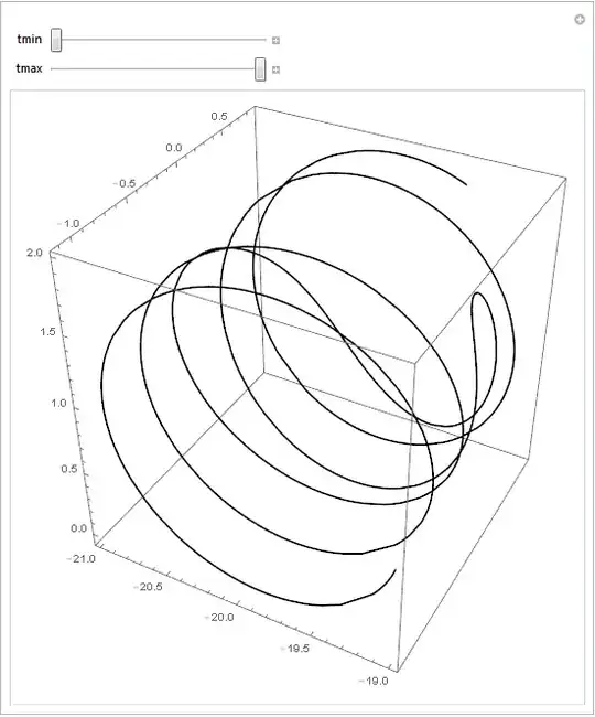
which gives:

However, though I increased the PlotPoints option to 3000, there still remained a defect at the upper left corner of the spring:

How can I obtain a smooth and normal tube version spring without such a defect?

Update 1

Per @belisarius suggestion, I tried the following:

p=ParametricPlot3D[{20 Cos[t]-((837+800 Cos[2 t]-35 Cos[12 t]+40 Sqrt[2] Cos[t] Sqrt[801+Cos[12 t]]) Cos[300 t]+480 Sin[t] Sin[6 t] Sin[300 t])/(-1637+35 Cos[12 t]-40 Sqrt[2] Cos[t] Sqrt[801+Cos[12 t]]),
20 Sin[t]+(4 (40 Cos[t]+Sqrt[2] Sqrt[801+Cos[12 t]]) (10 Cos[300 t] Sin[t]-3 Sin[6 t] Sin[300 t]))/(1637-35 Cos[12 t]+40 Sqrt[2] Cos[t] Sqrt[801+Cos[12 t]]),
Cos[6 t]+(480 Cos[300 t] Sin[t] Sin[6 t]+(1565+37 Cos[12 t]+40 Sqrt[2] Cos[t] Sqrt[801+Cos[12 t]]) Sin[300 t])/(-1637+35 Cos[12 t]-40 Sqrt[2] Cos[t] Sqrt[801+Cos[12 t]])},
{t,0,2Pi},PlotStyle->Directive[Orange,Opacity[1],Specularity[White,10]],
Boxed->False,Axes->False,ImageSize->500,
PlotPoints->100,Method->{Refinement->{ControlValue->Pi/360}}]/.Line[pts_,rest___]:>Tube[pts,0.1,rest];

and obtained:

problem persists though looks a little different.

Update 2

When I use the following equation per comments by @N.J.Evans, problem is solved:

    {20 Cos[t]+((59+100 Cos[t]^2+50 Cos[2 t]+10 Cos[t] Sqrt[418-18 Cos[12 t]]-9 Cos[12 t]) Cos[240 t EllipticE[-(9/100)]])/(209+10 Cos[t] Sqrt[418-18 Cos[12 t]]-9 Cos[12 t])+(60 Sin[t] Sin[6 t] Sin[240 t EllipticE[-(9/100)]])/(209+10 Cos[t] Sqrt[418-18 Cos[12 t]]-9 Cos[12 t]),
20 Sin[t]+(10 (20 Cos[t]+Sqrt[418-18 Cos[12 t]]) Cos[240 t EllipticE[-(9/100)]] Sin[t])/(209+10 Cos[t] Sqrt[418-18 Cos[12 t]]-9 Cos[12 t])-(3 (20 Cos[t]+Sqrt[418-18 Cos[12 t]]) Sin[6 t] Sin[240 t EllipticE[-(9/100)]])/(209+10 Cos[t] Sqrt[418-18 Cos[12 t]]-9 Cos[12 t]),
(Cos[6 t] (209+10 Cos[t] Sqrt[418-18 Cos[12 t]]-9 Cos[12 t])-10 (6 Cos[240 t EllipticE[-(9/100)]] Sin[t] Sin[6 t]+(20+Cos[t] Sqrt[418-18 Cos[12 t]]) Sin[240 t EllipticE[-(9/100)]]))/(209+10 Cos[t] Sqrt[418-18 Cos[12 t]]-9 Cos[12 t])}

So it is the wrong equation that causes the defect.

thank you all for suggestions!

Try using Method -> {Refinement -> {ControlValue -> 1 Degree} as in http://mathematica.stackexchange.com/a/8490/193 — Dr. belisarius, Aug 21 '15 at 06:22
thanks! from the link you posted, such Refinement method works similar to that of increasing the PlotPoints, and does not seem to resolve the problem in my test with ControlValue->Pi/360 — LCFactorization, Aug 21 '15 at 06:58
"does not seem to resolve the problem" - can you then include a picture in your post? — J. M.'s missing motivation, Aug 21 '15 at 09:54
Are you sure it's a problem with plot? The expressions for x[t],y[t],z[t] all act funny near pi. — N.J.Evans, Aug 21 '15 at 12:11
@LCFactorization , you could always leave it and claim it's a plot of a phone cord from back when phones had cords. That little squiggle always seemed to be in there somewhere. — N.J.Evans, Aug 21 '15 at 13:18

score 3 · Accepted Answer · answered Aug 22 '15 at 13:23

In order to study that region where you get the defect try

f[t_] := {20 Cos[
     t] - ((837 + 800 Cos[2 t] - 35 Cos[12 t] + 
         40 Sqrt[2] Cos[t] Sqrt[801 + Cos[12 t]]) Cos[300 t] + 
      480 Sin[t] Sin[6 t] Sin[300 t])/(-1637 + 35 Cos[12 t] - 
      40 Sqrt[2] Cos[t] Sqrt[801 + Cos[12 t]]), 
  20 Sin[t] + (4 (40 Cos[t] + 
        Sqrt[2] Sqrt[801 + Cos[12 t]]) (10 Cos[300 t] Sin[t] - 
        3 Sin[6 t] Sin[300 t]))/(1637 - 35 Cos[12 t] + 
      40 Sqrt[2] Cos[t] Sqrt[801 + Cos[12 t]]), 
  Cos[6 t] + (480 Cos[300 t] Sin[t] Sin[
        6 t] + (1565 + 37 Cos[12 t] + 
         40 Sqrt[2] Cos[t] Sqrt[801 + Cos[12 t]]) Sin[
        300 t])/(-1637 + 35 Cos[12 t] - 
      40 Sqrt[2] Cos[t] Sqrt[801 + Cos[12 t]])}

and then wrap it in a Manipulate where you can control the range of the plot

Manipulate[
 ParametricPlot3D[f[t],

  {t, tmin, tmax},

  PlotStyle -> Black,
  Boxed -> True,
  Axes -> True,
  ImageSize -> 500,
  PlotPoints -> 100
  ],
 {{tmin, 0}, 0, 2 \[Pi]},
 {{tmax, 2 \[Pi]}, 0, 2 \[Pi]}
 ]

This results in

Mathematica graphics

Then narrow the range to between 3.1 and 3.2

Mathematica graphics

You can continue on in this manner and increase the PlotPoints and you always see the squiggle.

Are you sure it isn't related to the equation?

It is because of the wrong equation. thank you1 – LCFactorization Aug 22 '15 at 14:43 — LCFactorization, Aug 22 '15 at 14:43

How can I fix a defect in the 3D graphics rendering of a coiled tube?

1 Answers1