Why do I get an empty plot?

Question

I have the following code:

AlphaCovarianceMatrix = 1/8*{{3, 0, 1}, {0, 2, 0}, {1, 0, 3}};
BetaCovarianceMatrix[2 θ_] := 
  1/8 {{-2 Cos[2 θ], Sqrt[2] Sin[2 θ], 
     0}, {Sqrt[2] Sin[2 θ], 0, Sqrt[2] Sin[2 θ]}, {0, 
     Sqrt[2] Sin[2 θ], 2 Cos[2 θ]}};
GammaCovarianceMatrix[4 θ_] := 
  1/8 {{Cos[
      4 θ], -Sqrt[2] Sin[4 θ], -Cos[
       4 θ]}, {-Sqrt[2] Sin[4 θ], -2 Cos[4 θ], 
     Sqrt[2] Sin[4 θ]}, {-Cos[4 θ], 
     Sqrt[2] Sin[4 θ], Cos[4 θ]}};
Cvol[mu_, n_] := 
  AlphaCovarianceMatrix + (2 n)/(n + 1) BetaCovarianceMatrix[2 mu] + (
    n (n - 1))/((n + 1) (n + 2)) GammaCovarianceMatrix[4 mu];
B[n_] := Eigenvalues[Cvol[μ, n]];
Plot[{B[n][[1]], B[n][[2]], B[n][[3]]}, {n, 0, 50}, 
 PlotLegends -> {"λ1", "λ2", "λ3"}]

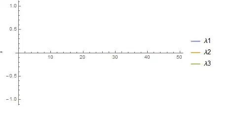
And I get the following empty plot:
In order to find the reason, I have checked some of the issues suggested by common pitfalls and I see that everything is calculated normally.

B[n]
(*
{(1 + 2 n)/(2 (1 + n) (2 + n)), (
 3 + 4 n + 2 n^2 - Sqrt[1 + 4 n + 20 n^2 + 16 n^3 + 4 n^4])/(
 4 (1 + n) (2 + n)), (
 3 + 4 n + 2 n^2 + Sqrt[1 + 4 n + 20 n^2 + 16 n^3 + 4 n^4])/(
 4 (1 + n) (2 + n))}
*)
B[0]
(*{1/2, 1/4, 1/4}*)

When I write the code as follows: (I don't consider any argument for B)

B = Eigenvalues[Cvol[μ, n]];
Plot[{B[[1]], B[[2]], B[[3]]}, {n, 0, 50}, 
 PlotLegends -> {"λ1", "λ2", "λ3"}]

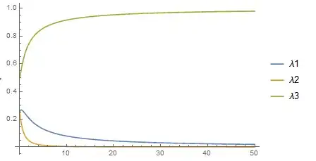
Everything's OK and the plot is done normally!!

Could you suggest me what the problem is?

Try Plot[Evaluate@{B[n][[1]], B[n][[2]], B[n][[3]]}, {n, 0, 50}, PlotLegends -> {"\[Lambda]1", "\[Lambda]2", "\[Lambda]3"}] or Plot[{B[n][[1]], B[n][[2]], B[n][[3]]}, {n, 0, 50}, PlotLegends -> {"\[Lambda]1", "\[Lambda]2", "\[Lambda]3"}, Evaluated -> True]. — Karsten7, Oct 18 '15 at 21:31
Or just Plot[Evaluate@B[n], {n, 0, 50}, PlotLegends -> {"\[Lambda]1", "\[Lambda]2", "\[Lambda]3"}]. — Karsten7, Oct 18 '15 at 21:34

Bob Hanlon · Answer 1 · 2015-10-19T00:17:07.807

AlphaCovarianceMatrix = 1/8*{{3, 0, 1}, {0, 2, 0}, {1, 0, 3}};
BetaCovarianceMatrix[2 θ_] := 
  1/8 {{-2 Cos[2 θ], Sqrt[2] Sin[2 θ], 
     0}, {Sqrt[2] Sin[2 θ], 0, Sqrt[2] Sin[2 θ]}, {0, 
     Sqrt[2] Sin[2 θ], 2 Cos[2 θ]}};
GammaCovarianceMatrix[4 θ_] := 
  1/8 {{Cos[
      4 θ], -Sqrt[2] Sin[4 θ], -Cos[
       4 θ]}, {-Sqrt[2] Sin[4 θ], -2 Cos[4 θ], 
     Sqrt[2] Sin[4 θ]}, {-Cos[4 θ], 
     Sqrt[2] Sin[4 θ], Cos[4 θ]}};
Cvol[mu_, n_] := 
  AlphaCovarianceMatrix + (2 n)/(n + 1) BetaCovarianceMatrix[
     2 mu] + (n (n - 1))/((n + 1) (n + 2)) GammaCovarianceMatrix[4 mu];
B[n_Integer] := Eigenvalues[Cvol[μ, n]];

ListLinePlot[Evaluate[Transpose[B /@ Range[0, 50]]], 
 PlotLegends -> (Subscript[λ, #] & /@ Range[3]),
 DataRange -> {0, 50}]

For non-integer values of n

Clear[B];

B[n_] := Eigenvalues[Cvol[μ, Rationalize[n]]] // ToRadicals // N;

ListLinePlot[Evaluate[Transpose[B /@ Range[0, 50, .25]]], 
 PlotLegends -> (Subscript[λ, #] & /@ Range[3]), DataRange -> {0, 50}]

Why do I get an empty plot?

1 Answers1