Finding the eigenvalues for the Schrödinger equation is really similar to finding the eigenvalues for the wave equation. You start with your differential equation
$$\left[-\frac{1}{2}\nabla'^2 + V(r)\right]\psi(\mathbf{r}) = E' \psi(\mathbf{r})$$
where we did the change of variable $(x,y,z) \rightarrow (a_0 x, a_0 y, a_0 z)$, with $a_0 \equiv 1$ Bohr, $E'= E/E_0$, $E_0 \equiv \frac{\hbar^2}{m_e a_0^2}$. The equation is written in a system of units that is more suitable for numerics ($m_e=1, \hbar=1, e=1$).
The more straightforward approach is to discretize the operator with finite differences and find the eigenvalues. An example for the particle in a box, written in Python is here:
from __future__ import division, print_function
import numpy as np
from scipy.sparse import diags
from scipy.sparse.linalg import eigsh
L = 2
N = 1000
dx = L/(N-1)
H = diags([-2., 1., 1.], [0,-1, 1], shape=(N, N))/dx**2
vals, vecs = eigsh(-0.5*H, which='SA')
print(np.round(vals, 6))
print(np.round([(nnp.pi/L)*2/2 for n in range(1,6)], 6))
Where the results are
[  1.228775   4.915086  11.058899  19.660151  30.71876   44.234615]
[  1.233701   4.934802  11.103305  19.739209  30.842514  44.41322 ]
The analytic solution for this normalized case is $E' = \frac{n^2 \pi^2}{2L^2}$. That is printed in the second line, the agreement is "adequate", and if we discretize more, the error is smaller.
In the case of an "arbitrary" potential, we can do the same, just adding the potential energy
from __future__ import division, print_function
import numpy as np
from scipy.sparse import diags
from scipy.sparse.linalg import eigsh
import matplotlib.pyplot as plt
L = 2*np.pi
N = 501
x = np.linspace(0, L, N)
dx = x[1] - x[0]
T = -0.5diags([-2., 1., 1.], [0,-1, 1], shape=(N, N))/dx2
U_vec = np.sin(x)*2
U = diags([U_vec], [0])
H = T + U
vals, vecs = eigsh(H, which='SM')
print(np.round(vals, 6))
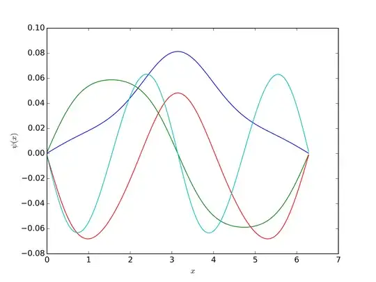
for k in range(4):
vec = vecs[:, k]
mag = np.sqrt(np.dot(vecs[:, k],vecs[:, k]))
vec = vec/mag
plt.plot(x, vec, label=r"$n=%i$"%k)
plt.xlabel(r"$x$")
plt.ylabel(r"$\psi(x)$")
plt.savefig("eigenvectors.png", dpi=600)
plt.legend()
plt.show()
with results
[ 0.545762 1.227567 1.657063 2.470791 3.610032 4.970446]
That I have no idea if are good or not. The eigenvectors make sense, though
Comparing to the Ritz method (with 10 sine functions)
[0.4111, 0.8299, 1.6696, 2.83472, 4.3342, 6.16726]
it makes sense
Another option is to base your formulation on a variational approach. In this case, you start from the variational formulation of the problem, i.e.
$$ \Pi[u] = \int_\Omega\left[\frac{1}{2}\nabla u^*(\mathbf{r}) \cdot\nabla u(\mathbf{r}) + u^*(\mathbf{r})(V(\mathbf{r})-E)u(\mathbf{r})\right] d\Omega$$
That has as components, the Hamiltonian
$$H[u] = \int_\Omega\left[\frac{1}{2}\nabla u^*(\mathbf{r}) \cdot\nabla u(\mathbf{r}) + u^*(\mathbf{r})V(\mathbf{r})u(\mathbf{r})\right] d\Omega$$
and the overlap operator
$$S[u] = \int_\Omega\left[u^*(\mathbf{r})u(\mathbf{r})\right] d\Omega \enspace .$$
The solution for this system is at a stationary point of the functional. For an approximate solution of the form $\hat{u} = \sum_i^N c_i f_i(x)$, we obtain an approximation of the functionals. And we can form the eigenvalue problem
$$[\hat{H}]\lbrace c\rbrace = E [\hat{S}]\lbrace c\rbrace$$
with $\hat{H}_{ij} = \frac{H}{\partial c_i \partial c_j}$ and $\hat{S}_{ij}=\frac{S}{\partial c_i \partial c_j} \enspace.$ This approach is a Ritz method and it is similar to the one used in Hartree-Fock Methods and Density Functional Theory (DFT), and also to Finite Element Methods.
I solved for a potential $V(x) = x(2\pi - x)$ analytically using Sympy here, with eigenvalues
[ 5.72324464, 9.04413044, 11.55005606, 14.95945642, 19.85359933]
Using 20 functions I found these values (not in Sympy though)
[5.717086647332907,9.033168327518542,11.52268082000659,14.84436075114633,19.25485456061611]
that are really close.