Draw a spiral on a sphere

Question

My goal is to visualize damped magnetic precession.

Wikipedia features an image, but it doesn't quite capture one essential constraint. Namely, that the magnetization M should be normalized. So the curve shown in the following picture should lie on the sphere.

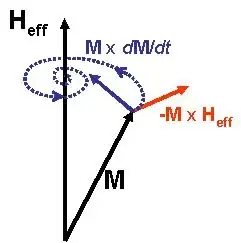
So what I want to show is:

• The vectors M and H_eff with M on the sphere.
• A spiral lying on a sphere.
• -M x H_eff being orthogonal to M and H_eff
• M x dM/dt pointing towards H_eff (This is not exactly correct, but rather an approximation).

The tangent of the spiral at the endpoint of M should be a linear combination of MxdM/dt and -MxH_eff (to be more exact: alpha MxdM/dt - MxH_eff for some positive alpha), so the picture on Wikipedia looks fine concerning this requirement.

I have found a similar picture in the following answer: https://tex.stackexchange.com/a/56617/50081

How can this be achieved with any of the modern plotting tools for LaTeX?

Edit: As Christian pointed out one could start by generating the spiral via projection of a flat spiral. This is my first try using pgfplots.

\documentclass{minimal}
\usepackage{tikz}
\usepackage{pgfplots}
\begin{document}
\begin{tikzpicture}
\xdef\w{10}

\begin{axis}[%
    axis equal,
    axis lines = none,
    xlabel = {$x$},
    ylabel = {$y$},
    zlabel = {$z$},
    enlargelimits = 0.5,
    ticks=none,
]
    \addplot3[%
        opacity = 0.2,
        surf,
        z buffer = sort,
        samples = 21,
        variable = \u,
        variable y = \v,
        domain = 0:180,
        y domain = 0:360,
    ]
    ({cos(u)*sin(v)}, {sin(u)*sin(v)}, {cos(v)});

    \addplot3+[color=blue,domain=0:4*pi, samples=100, samples y=0,no marks, smooth](
        {x*cos(deg(x))/sqrt(\w*\w+x*x)},
        {x*-sin(deg(x))/sqrt(\w*\w+x*x)},
        {\w/sqrt(\w*\w+x*x)}
        );
\end{axis}
\end{tikzpicture}
\end{document}

Answer 1

Here's an attempt using Asymptote. I took literally your statement that "any spirally shape" would be okay. To compile it, save the code below in a file called (e.g.) filename.tex and then run pdflatex --shell-escape filename. (Also, make sure you have Asymptote installed.)

\documentclass[margin=10pt,convert]{standalone}
\usepackage{asypictureB}
\begin{document}
\begin{asypicture}{name=sphere_spiral}
    settings.outformat = "png";
    settings.render = 16;
    import graph3;
    size(10cm);

    triple eye = (5,2,3);
    currentprojection=orthographic(eye);

    surface hemisphere = surface(Arc(X,-X,c=O,normal=Z,n=16), c=O, axis=X, angle1=0, angle2=180);
    draw(shift(-5 eye)*hemisphere, material(white + opacity(0.5), emissivepen=0.2 white));

    usepackage("amsmath");  //for \text command
    draw(O -- 1.6Z, arrow=Arrow3, L=Label("$H_{\text{eff}}$", align=W, position=EndPoint));

    real theta(real t) { return t/20; }
    real phi(real t) { return -t + 1; }
    real r(real t) { return 1; }
    triple F(real t) { return polar(r(t), theta(t), phi(t)); }

    path3 spiral = reverse(graph(F, 0, 4pi, operator ..));
    draw(spiral, blue + dotted + linewidth(1pt));

    real t = 0.1;
    triple arrowpos = point(spiral, reltime(spiral, t));
    add(arrow(arrowhead=TeXHead2(normal=arrowpos), g=spiral, p=invisible, 
        arrowheadpen=emissive(blue), FillDraw(blue), position=Relative(t)));

    t = 0.7;
    arrowpos = point(spiral, reltime(spiral, t));
    add(arrow(arrowhead=TeXHead2(normal=arrowpos), g=spiral, p=invisible, 
        arrowheadpen=emissive(blue), FillDraw(blue), position=Relative(t)));

    triple M = point(spiral, 0);
    draw(O -- M, arrow=Arrow3, L=Label("$M$", position=MidPoint));
    draw(shift(M) * (O -- 0.5 cross(-M, Z)), red, arrow=Arrow3, L=Label("$-M \times H_{\text{eff}}$", position=MidPoint));
    triple dMdt = dir(spiral,0);
    triple crossprod = cross(M, dMdt);
    draw(shift(M) * (O -- 0.5 crossprod), blue, arrow=Arrow3, L=Label("$M \times \frac{dM}{dt}$", position=MidPoint));
\end{asypicture}
\end{document}

The result:

Answer 2

The figure is interesting, so I give another simple Asymptote solution. Starting with a spiral, I project on the Oxy plane to get the blue; and project on the sphere to get the red one.

Of course, the projection of the red is exactly the blue, by the construction.

// http://asymptote.ualberta.ca/
unitsize(2cm);
import graph3;
currentprojection=orthographic(3,1.5,1.2,zoom=.9);
//currentprojection=orthographic(Z,zoom=.9);
real r(real t) {return .01+t/30;}
real x(real t) {return r(t)cos(t);}
real y(real t) {return r(t)sin(t);}
real z(real t) {return sqrt(1-r(t)*r(t));}
real z0(real t) {return 0;}
path3 p=graph(x,y,z,0,8pi,operator..);
path3 p0=graph(x,y,z0,0,8pi,operator..);
draw(p,red,Arrow3);
draw(p0,blue,Arrow3);
draw(unithemisphere,yellow+opacity(.5));
zaxis3("$H_{\rm{eff}}$",zmax=1.5,Arrow3);

Answer 3

Well, I agree with Black Mild's answer, the figure is very interesting. So I'm adding a TikZ version too.

For this I defined two simple \pics, one for the spiral and another one for the sphere parts (visible and non-visible).

\documentclass[tikz,border=1.618]{standalone}
\usetikzlibrary{3d,perspective}
\tikzset
{
  declare function={
    rho(\x)=0.05\x;
    theta(\x)=deg(-0.5pi\x);
    z(\x)=sqrt(abs(1-rho(\x)^2);},
  my ball/.style={shading=ball,ball color=green,fill opacity=0.5,draw=green!50!black},
  % SPIRAL
  pics/spiral/.style n args={3}{% #1:#2 --> domain in [0:20], #3 --> 0=draw proyection, 1=draw 3d
     /tikz/transform shape,code=%
    {\draw[pic actions] plot[domain=#1:#2,samples={int(40(#2-#1))+1}]
                        ({rho(\x)cos(theta(\x))},{rho(\x)sin(theta(\x))},{#3z(\x)});}},
  % SPHERE
  pics/sphere/.style={% #1 --> -1=back, 1=front
       /tikz/transform shape,code=%
      {\draw[pic actions,rotate around z=-45] (1,0) arc (0:#1180:1) arc (0:180:1cm);}},
}
\begin{document}
\begin{tikzpicture}[isometric view,rotate around z=180,
                    line cap=round,line join=round,scale=2]
% x,y axes
\draw[-latex] (0,0,0) -- (2,0,0) node[left]  {\strut$x$};
\draw[-latex] (0,0,0) -- (0,2,0) node[right] {\strut$y$};
% spiral (projection)
\pic [gray]   {spiral={0}{20}{0}};
% sphere (back)
\pic[my ball] {sphere=-1};
% spriral (back)
\pic [gray]   {spiral={16.75}{18.3}{1}};
% z axis (below)
\draw         (0,0,0) -- (0,0,1);
% sphere (front)
\pic[my ball] {sphere=1};
% spiral (front)
\pic[blue]    {spiral={0}{16.75}{1}};
\pic[blue]    {spiral={18.3}{20}{1}};
% z axis (above)
\draw[-latex] (0,0,1) -- (0,0,2) node[above] {$z$};
\end{tikzpicture}
\end{document}