0

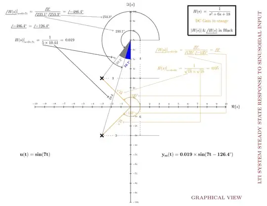
I have made the attached picture in 2018. It full filled its purpose for my tutorial. Now I want to add it into my lecture notes. But the problem is that it is using overlay when I scale it down even using transform shape, the things get distorted. If somebody can help to scale the picture down so it can fit at any size like scale to 0.7 without distorting it. I remember I spend lot of time to make it as I was and still learning pgfplots. The complete running code is attached here.

\documentclass[a3paper,landscape]{article}
\usepackage{tikz}
\usetikzlibrary{shapes.misc}
\usetikzlibrary{arrows.meta}
\usepackage{steinmetz}
\usepackage{xcolor}
\usepackage{background}

\usepackage{amsmath,mleftright} \usepackage{xparse}

\NewDocumentCommand{\evalat}{sO{\big}mm}{%

\IfBooleanTF{#1} {\mleft. #3 \mright|{#4}} {#3#2|{#4}}% }

\backgroundsetup{% scale=1, %% change accordingly angle=0, %% change accordingly opacity=.5, %% change accordingly color =black, %% change accordingly contents={ % \begin{tikzpicture}[remember picture,overlay] % \node at (-11.5,-8.5) {\includegraphics[width=0.25\textwidth]{seal.png}}; %% yshift and xshift for example only % \end{tikzpicture} } }

\begin{document} \thispagestyle{empty}

\begin{tikzpicture}[remember picture, overlay] \node [shift={(0cm,0cm)}] at (current page.center) {% \begin{tikzpicture}

\begin{scope}[thick,font=\scriptsize]
% Axes:
% Are simply drawn using line with the `->` option to make them arrows:
% The main labels of the axes can be places using `node`s:
\draw [->] (-10,0) -- (10,0) node [xshift=1cm]  {\large $\Re\{s\}$};
\draw [->] (0,-10) -- (0,10) node [yshift=0.7cm] {\large $\Im\{s\}$};

% Axes labels:
% Are drawn using small lines and labeled with `node`s. The placement can be set using options
\iffalse% Single

% If you only want a single label per axis side: \draw (1,-3pt) -- (1,3pt) node [above] {$1$}; \draw (-1,-3pt) -- (-1,3pt) node [above] {$-1$}; \draw (-3pt,1) -- (3pt,1) node [right] {$i$}; \draw (-3pt,-1) -- (3pt,-1) node [right] {$-i$}; \else% Multiple % If you want labels at every unit step: \foreach \n in {-10,...,-1,1,2,...,10}{% \draw (\n,-3pt) -- (\n,3pt) node [above] {$\n$}; \draw (-3pt,\n) -- (3pt,\n) node [right] {$\n i$}; } \fi \end{scope} % The circle is drawn with (x,y) circle (radius) % You can draw the outer border and fill the inner area differently. % Here I use gray, semitransparent filling to not cover the axes below the circle % \path [draw=none,fill=gray,semitransparent] (+1,-1) circle (3); % Place the equation into the circle: % \node [below right,darkgray] at (+1,-1) {$|z-1+i| \leq 3$}; \node[cross out,draw=black, line width=1mm] at (-3,3) {}; \node[cross out,draw=black, line width=1mm] at (-3,-3) {}; \draw (0,7) -- (-3,3) node[midway,above=8pt,left=1pt, rotate=45] {$5$}; \draw (0,7) -- (-3,-3) node at (-1.8,1) [above=12pt,left=2pt, rotate=65] {$10.4$}; \draw (0,7) -- (3,7); \draw [thick,->] (1,7) arc (0:233.13:1cm) node[midway,above=1pt,left=1pt] {$233.1^{\circ}$}; \draw [thick,->] (3,7) arc (0:253.3:3cm) node[midway,above=1pt,left=1pt] {$253.3^{\circ}$}; \draw [dashed] (-3,3) -- (-2.2,3) node [xshift=10pt] {$3$}; \draw [dashed] (0,3) -- (-1.4,3); \draw [dashed] (-3,-3) -- (-1.7,-3) node [xshift=5pt] {$3$}; \draw [dashed] (0,-3) -- (-1.4,-3); \fill [blue] (0,7) -- (0,5) arc (-90:-106.7:2cm) -- cycle node [rotate=45] at (-0.35,4.5) {$\mathbf{16.7^{\circ}}$}; \fill [gray] (0,7) -- (-0.57,5.08) arc (-106.7:-126.87:2cm) -- cycle node [rotate=45] at (-1.2,4.8) {$\mathbf{20.2^{\circ}}$}; \draw (0,3) -- (3,3); \draw [<-, dashed] (1,7) -- (1,5.6) node [yshift=-15pt] {$4$}; \draw [->,dashed] (1,4.5) -- (1,3); \draw [<-, dashed] (1,3) -- (1,-0.5) node [yshift=-15pt] {$6$}; \draw [->,dashed] (1,-1.5) -- (1,-3); \draw (0,-3) -- (3,-3); \node at (-9,7) {\large $\evalat{H(s)}{s=0+7i}:=:\dfrac{1}{5 \times 10.44}:=:0.019$}; \draw [thick,->] (-9.2,6.5) -- (-1.9,5.2); \draw [thick,->] (-8,6.5) -- (-2.3,1); \node at (-9,10) {\large $\evalat{\phase{H(s)}}{s=0+7i}:=:\dfrac{\phase{0^{\circ}}}{\phase{233.1^{\circ}}:\phase{253.3^{\circ}}}:=:\phase{-486.4^{\circ}}$}; \node at (-10.5,8.5) {\large $\phase{-486.4^{\circ}}:=: \phase{-126.4^{\circ}}$}; \draw [->] (-7.3,9.6) -- (-3,9.4); \draw [->] (-9,9.4) -- (-1.8,8); \node at (-10,-5) {\Large $\mathbf{u(t)=sin(7t)}$}; \node at (7,-5) {\Large $\mathbf{y_{ss}(t)=0.019 \times sin(7t-126.4^{\circ})}$}; \draw [thick, orange] (0,0) -- (-3,3) node at (-1,1) [above=8pt,left=-5pt, rotate=-45] {$\sqrt{18}$}; \draw [thick, orange] (0,0) -- (-3,-3) node at (-1,-1) [below=8pt,left=-5pt, rotate=45] {$\sqrt{18}$}; \draw [thick, ->, orange] (1,0) arc (0:135:1cm) node[midway,above=8pt,left=-15pt] {$135^{\circ}$}; \draw [thick, ->, orange] (1,0) arc (0:-135:1cm) node[midway,above=8pt,left=-5pt] {$-135^{\circ}$}; \node [orange] at (6,4) {\large $\evalat{H(s)}{s=0+0i}:=:\dfrac{1}{\sqrt{18} \times \sqrt{18}}:=:0.0\bar{5}$}; \draw [orange, ->] (6,3.5) -- (-0.65,1.5); \draw [orange, ->] (7.3,3.5) -- (7.3,-1.6) -- (-0.8,-1.6); \node [orange] at (6,6) {\large $\color{orange}\evalat{\phase{{\color{orange}{H(s)}}}}{s=0+0i}:=:\color{orange}\dfrac{\color{orange}\phase{{\color{orange}{0^{\circ}}}}}{\color{orange}\phase{{\color{orange}{135^{\circ}}}}:\phase{{\color{orange}{-135^{\circ}}}}}:=:\color{orange}\phase{{\color{orange}{0^{\circ}}}}$}; \draw [orange, ->] (8.2,5.6) -- (10,5.5) -- (10,-0.65) -- (0.5,-0.65); \draw [orange, ->] (6,5.3) -- (9.5,4.5) -- (9.5,1.15) -- (0.8,1.15); \draw [line width=1mm] (6,7.5) -- (6,10.6) -- (11,10.6) -- (11,7.5) -- (6,7.5); \node at (8.5,10) {\large $H(s):=:\dfrac{1}{s^2+6s+18}$}; \node [orange] at (8.5,9) {\large DC Gain in orange}; \node at (8.5,8) {\large $|H(s)|:&amp;:\phase{H(s)}$ in Black}; \node [rotate=90, red!40!gray] at (13.5,1) {\Large

\textbf{LTI SYSTEM STEADY STATE RESPONSE TO SINUSOIDAL INPUT}}; \node [purple!40!gray] at (9,-9.5) {\Large \textbf{GRAPHICAL VIEW}}; \end{tikzpicture} }; % % Draw a page border % \draw (current page.north west) rectangle (current page.south east); \end{tikzpicture}

\end{document}
picture

Bernard
  • 271,350

1 Answers1

2

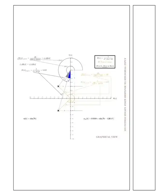
Using the package adjustbox and

with (for your notes) \documentclass{article}

starting the picture as

\begin{tikzpicture}[remember picture, overlay]
    \node [shift={(0cm,0cm)}]  at (current page.center)
    {%      
    \begin{adjustbox}{width=4.5in}% % added <<<<<<<
            \begin{tikzpicture}

and ending

    \node [purple!40!gray] at (9,-9.5) {\Large \textbf{GRAPHICAL VIEW}};
        \end{tikzpicture}   
    \end{adjustbox} % added <<<<<<<<<<
    };
    % % Draw a page border
    % \draw (current page.north west) rectangle (current page.south east);
\end{tikzpicture}

you will get

b

No discernible distortions with smaller widths.

This is the complete code.

\documentclass{article}
\usepackage{tikz}
\usetikzlibrary{shapes.misc}
\usetikzlibrary{arrows.meta}
\usepackage{steinmetz}
\usepackage{xcolor}
\usepackage{background}

\usepackage{amsmath,mleftright} \usepackage{xparse}

\NewDocumentCommand{\evalat}{sO{\big}mm}{%
\IfBooleanTF{#1} {\mleft. #3 \mright|{#4}} {#3#2|{#4}}% }

\backgroundsetup{% scale=1, %% change accordingly angle=0, %% change accordingly opacity=.5, %% change accordingly color =black, %% change accordingly contents={ % \begin{tikzpicture}[remember picture,overlay] % \node at (-11.5,-8.5) {\includegraphics[width=0.25\textwidth]{seal.png}}; %% yshift and xshift for example only % \end{tikzpicture} } }

\usepackage{showframe} % show the margin <<<<<<<<<<<<<<<<<<

\usepackage{adjustbox} % added <<<<<<<<<<<<<<<<<<<<<<<

\begin{document} \thispagestyle{empty}

\begin{tikzpicture}[remember picture, overlay]
    \node [shift={(0cm,0cm)}]  at (current page.center)
    {%      
    \begin{adjustbox}{width=4.5in}% % added &lt;&lt;&lt;&lt;&lt;&lt;&lt;
            \begin{tikzpicture}

            \begin{scope}[thick,font=\scriptsize]
                % Axes:
                % Are simply drawn using line with the `-&gt;` option to make them arrows:
                % The main labels of the axes can be places using `node`s:
                \draw [-&gt;] (-10,0) -- (10,0) node [xshift=1cm]  {\large $\Re\{s\}$};
                \draw [-&gt;] (0,-10) -- (0,10) node [yshift=0.7cm] {\large $\Im\{s\}$};

                % Axes labels:
                % Are drawn using small lines and labeled with `node`s. The placement can be set using options
                \iffalse% Single
                % If you only want a single label per axis side:
                \draw (1,-3pt) -- (1,3pt)   node [above] {$1$};
                \draw (-1,-3pt) -- (-1,3pt) node [above] {$-1$};
                \draw (-3pt,1) -- (3pt,1)   node [right] {$i$};
                \draw (-3pt,-1) -- (3pt,-1) node [right] {$-i$};
                \else% Multiple
                % If you want labels at every unit step:
                \foreach \n in {-10,...,-1,1,2,...,10}{%
                    \draw (\n,-3pt) -- (\n,3pt)   node [above] {$\n$};
                    \draw (-3pt,\n) -- (3pt,\n)   node [right] {$\n i$};
                }
                \fi
            \end{scope}
            % The circle is drawn with `(x,y) circle (radius)`
            % You can draw the outer border and fill the inner area differently.
            % Here I use gray, semitransparent filling to not cover the axes below the circle
            % \path [draw=none,fill=gray,semitransparent] (+1,-1) circle (3);
            % Place the equation into the circle:
            % \node [below right,darkgray] at (+1,-1) {$|z-1+i| \leq 3$};
            \node[cross out,draw=black, line width=1mm] at (-3,3) {};
            \node[cross out,draw=black, line width=1mm] at (-3,-3) {};
            \draw (0,7) -- (-3,3) node[midway,above=8pt,left=1pt, rotate=45] {$5$};
            \draw (0,7) -- (-3,-3) node at (-1.8,1) [above=12pt,left=2pt, rotate=65] {$10.4$};
            \draw (0,7) -- (3,7);
            \draw [thick,-&gt;] (1,7) arc (0:233.13:1cm) node[midway,above=1pt,left=1pt] {$233.1^{\circ}$};
            \draw [thick,-&gt;] (3,7) arc (0:253.3:3cm) node[midway,above=1pt,left=1pt] {$253.3^{\circ}$};
            \draw [dashed] (-3,3) -- (-2.2,3) node [xshift=10pt] {$3$};
            \draw [dashed] (0,3) -- (-1.4,3);
            \draw [dashed] (-3,-3) -- (-1.7,-3) node [xshift=5pt] {$3$};
            \draw [dashed] (0,-3) -- (-1.4,-3);
            \fill [blue]  (0,7) -- (0,5) arc (-90:-106.7:2cm) -- cycle node [rotate=45] at (-0.35,4.5) {$\mathbf{16.7^{\circ}}$};
            \fill [gray] (0,7) -- (-0.57,5.08) arc (-106.7:-126.87:2cm) -- cycle node [rotate=45] at (-1.2,4.8)     {$\mathbf{20.2^{\circ}}$};
            \draw (0,3) -- (3,3);
            \draw [&lt;-, dashed] (1,7) -- (1,5.6) node [yshift=-15pt] {$4$}; 
            \draw [-&gt;,dashed] (1,4.5) -- (1,3);
            \draw [&lt;-, dashed] (1,3) -- (1,-0.5) node [yshift=-15pt] {$6$}; 
            \draw [-&gt;,dashed] (1,-1.5) -- (1,-3);
            \draw (0,-3) -- (3,-3);
            \node at (-9,7) {\large $\evalat{H(s)}{s=0+7i}\:=\:\dfrac{1}{5 \times 10.44}\:=\:0.019$};
            \draw [thick,-&gt;] (-9.2,6.5) -- (-1.9,5.2);
            \draw [thick,-&gt;] (-8,6.5) -- (-2.3,1);
            \node at (-9,10) {\large        $\evalat{\phase{H(s)}}{s=0+7i}\:=\:\dfrac{\phase{0^{\circ}}}{\phase{233.1^{\circ}}\:\phase{253.3^{\circ}}}\:=\:\phase{-486.4^{\circ}}$};
            \node at (-10.5,8.5) {\large $\phase{-486.4^{\circ}}\:=\: \phase{-126.4^{\circ}}$};
            \draw [-&gt;] (-7.3,9.6) -- (-3,9.4);
            \draw [-&gt;] (-9,9.4) -- (-1.8,8);
            \node at (-10,-5) {\Large $\mathbf{u(t)=sin(7t)}$};
            \node at (7,-5) {\Large $\mathbf{y_{ss}(t)=0.019 \times sin(7t-126.4^{\circ})}$};
            \draw [thick, orange] (0,0) -- (-3,3) node at (-1,1) [above=8pt,left=-5pt, rotate=-45] {$\sqrt{18}$};
            \draw [thick, orange] (0,0) -- (-3,-3) node at (-1,-1) [below=8pt,left=-5pt, rotate=45] {$\sqrt{18}$};
            \draw [thick, -&gt;, orange] (1,0) arc (0:135:1cm) node[midway,above=8pt,left=-15pt] {$135^{\circ}$};
            \draw [thick, -&gt;, orange] (1,0) arc (0:-135:1cm) node[midway,above=8pt,left=-5pt] {$-135^{\circ}$};
            \node [orange] at (6,4) {\large $\evalat{H(s)}{s=0+0i}\:=\:\dfrac{1}{\sqrt{18} \times \ sqrt{18}}\:=\:0.0\bar{5}$};
            \draw [orange, -&gt;] (6,3.5) -- (-0.65,1.5);
            \draw [orange, -&gt;] (7.3,3.5) -- (7.3,-1.6) -- (-0.8,-1.6);
            \node [orange] at (6,6) {\large     $\color{orange}\evalat{\phase{{\color{orange}{H(s)}}}}{s=0+0i}\:=\:\color{orange}\dfrac{\color{orange}\phase{{\color{orange}{0^{\circ}}}}}{\color{orange}\phase{{\color{orange}{135^{\circ}}}}\:\phase{{\color{orange}{-135^{\circ}}}}}\:=\:\color{orange}\phase{{\color{orange}{0^{\circ}}}}$};
                \draw [orange, -&gt;] (8.2,5.6) -- (10,5.5) -- (10,-0.65) -- (0.5,-0.65);
            \draw [orange, -&gt;] (6,5.3) -- (9.5,4.5) -- (9.5,1.15) -- (0.8,1.15);
            \draw [line width=1mm] (6,7.5) -- (6,10.6) -- (11,10.6) -- (11,7.5) -- (6,7.5);
            \node at (8.5,10) {\large $H(s)\:=\:\dfrac{1}{s^2+6s+18}$};
            \node [orange] at (8.5,9) {\large DC Gain in orange};
            \node at (8.5,8) {\large $|H(s)|\:\&amp;\:\phase{H(s)}$ in Black};
            \node [rotate=90, red!40!gray] at (13.5,1) {\Large                  
            \textbf{LTI SYSTEM STEADY STATE RESPONSE TO SINUSOIDAL INPUT}};
            \node [purple!40!gray] at (9,-9.5) {\Large \textbf{GRAPHICAL VIEW}};
        \end{tikzpicture}   
    \end{adjustbox} % added &lt;&lt;&lt;&lt;&lt;&lt;&lt;&lt;&lt;&lt;
    };
    % % Draw a page border
    % \draw (current page.north west) rectangle (current page.south east);
\end{tikzpicture}   

\end{document}
Simon Dispa
  • 39,141