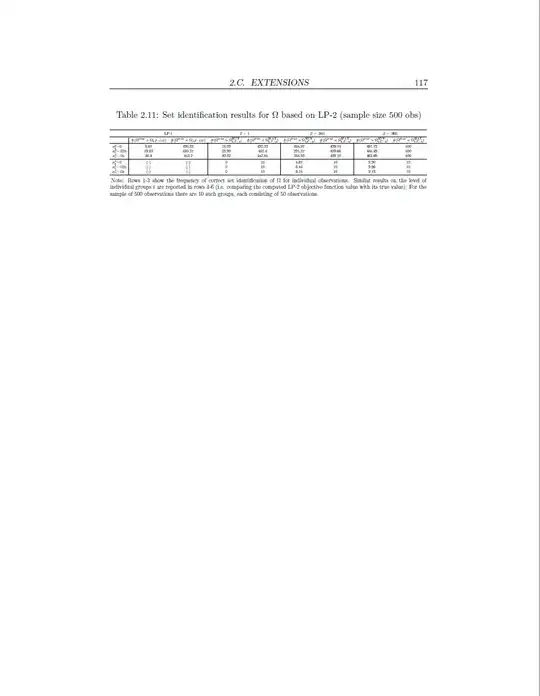
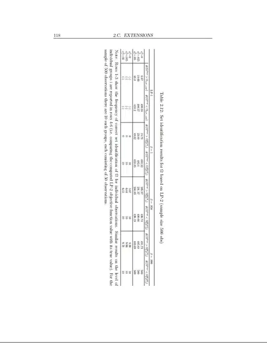
How to remove empty page created by sidewaystable in a threeparttable with resizebox (shrinking table does not work)?

Question

I am finalizing my PhD thesis. The last task remaining is to enlarge tables and figures so that they can be clearly viewed on smaller printed formats. I have one table which is hard to read when using a simple table environment (p.117 below). Therefore I want to include this as a sidewaystable (see p.118). However, this creates an empty page after the table (p. 119). Perhaps my table on p.118 is too big to put it on one page, so therefore I used the \resizebox command. Even when using for example \resizebox{0.3\textwidth}{!} the table on p.118 shrinks but the problem of the empty page remains. I have read answers to similar questions and understand that sidewaystable creates a page-wide float but none of these previous answers solved my problem. I've been trying to solve this for hours, reading through a bunch of questions related to sidewaystable. At this point I don't even know what it is I am doing wrong. Perhaps it has to do with mixing sidewaystable and threeparttable? I've played around with \FloatBarrier, \clearpage and \newpage but none of that seems to help... Any guidance is much appreciated.

Below you can find my preamble together with the code for pages 116-119:

Pre-amble:

\documentclass[10pt,twoside]{report}
\usepackage{appendix,amsmath,amscd,amssymb,amsfonts,amsthm,setspace,booktabs,pgfplotstable,a4wide,float,floatflt,bbm,tikz,pdflscape}
\usepackage{tikz,etoolbox,graphicx,chngpage,pdfpages,multirow,fancyhdr,verbatim,float,lscape,rotating,color, colortbl,longtable,graphicx,mathrsfs,eurosym,enumerate}
\usepackage[normalem]{ulem}
\usepackage[margin=1.75in]{geometry}
\usepackage{adjustbox}
\usepackage{refstyle}
\usepackage[colorlinks=true, citecolor=black, linkcolor=black, urlcolor=black,breaklinks]{hyperref}
\usepackage[round,authoryear]{natbib} 
\usepackage[flushleft]{threeparttable}
\usepackage[section]{placeins}
\usepackage{mathtools,subcaption,bm,arydshln,bookmark,chngcntr,titlesec}
\usetikzlibrary{positioning}
\newcommand{\npar}{\par \vspace{2.3ex plus 0.3ex minus 0.3ex}}
\setcounter{MaxMatrixCols}{10}
\begin{document}
\newcommand{\fra}[1]{\ensuremath{\frac{\partial #1}{\partial #2}}}
\raggedbottom
\pagenumbering{gobble}\clearpage
\chapter{Second chapter}
\input{chapter2} %The pages mentioned are inside the chapter2.tex file
\clearpage
\bibliographystyle{abbrvnat}
\bibliography{References_PhD}
\end{document}

Code for the pages 116-118:

p.116 (just some text and math symbols):

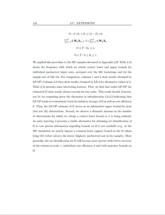
\begin{enumerate}
\item[] \begin{equation*} \text{Min/Max } \sum^{s}_{t=1} \Omega_{t \mid t \in i} 
\end{equation*}
\item[] subject to
\item[] \begin{center} $\forall t,s \in T: \hat{\theta_{t}} \mathbf{W_{t}X_{t}} + \Omega_{t} \leqslant \mathbf{W_{t}} (\left( \frac{Q_{t}}{Q_{s}} \right)^{\frac{1}{\gamma}} \mathbf{X_{s}}) + \Omega_{s}$.
\end{center}
\item[] \begin{center}
$\forall t: \beta*\theta_{t} \leq \hat{\theta_{t}} \leq (2-\beta)*\theta_{t}$
\end{center}
\item[] \begin{center}
$\sum^{T}_{t=1} \hat{\theta_{t}} \mathbf{W_{t} X_{t}} \geq \beta* \sum^{T}_{t=1} \theta_{t} \mathbf{W_{t} X_{t}}$
\end{center}
\item[] \begin{center} $\forall t \in T: \Omega_{t} \geq a$. \end{center}
\item[] \begin{center} $\forall t \in T: 0 \leq \hat{\theta_{t}} \leq 1$.
\end{center}
\end{enumerate}
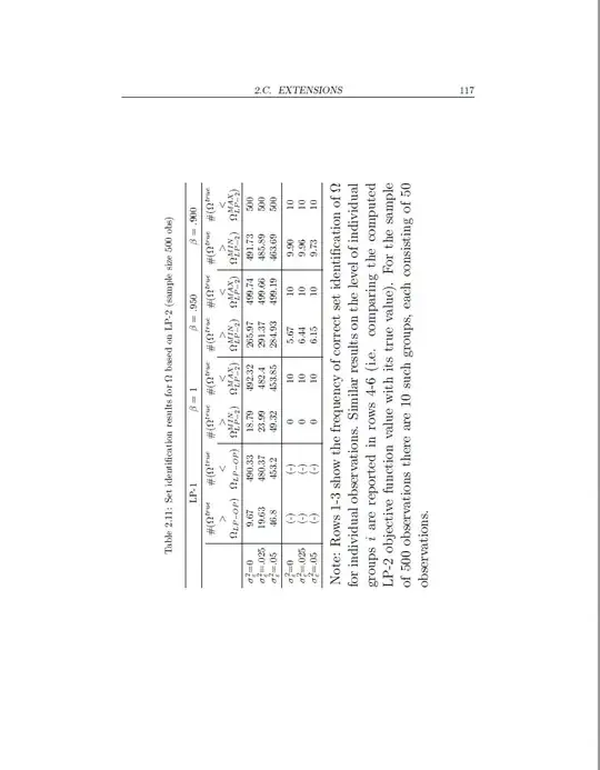
We applied this procedure to the MC samples discussed in Appendix \ref{MonteCarlo}. \autoref{MCboundsbeta} shows the frequency with which we obtain correct lower and upper bounds for individual unobserved input costs, averaged over the 200 bootstraps and for the sample size of 500 obs. For comparison, columns 1 and 2 show results obtained by LP-OP. Columns 3-8 then show results obtained by LP-2 for alternative values of $\beta$. \autoref{MCboundsbeta} presents some interesting features. First, we find that under LP-OP the estimated $\Omega$ value nearly always exceeds its true value. This result should, however, not be too surprising given the discussion in \autoref{identifomega} indicating that LP-OP tends to overestimate both the industry average of $\Omega$ as well as cost efficiency $\theta$. Thus, the LP-OP estimate of $\Omega$ serves as an informative upper bound for most (but not all) observations. Second, we observe a dramatic increase in the number of observations for which we obtain a correct lower bound as $\beta$ is being reduced. As such, lowering $\beta$ presents a viable alternative for obtaining set identification of $\Omega$ in case precise information regarding bounds on $\Omega$ is not available (e.g. in the MC simulation we merely impose a common lower (upper) bound on the $\Omega$ values lying 10\% below (above) the lowest (highest) unobserved cost in the sample). More generally, the set identification for $\Omega$ will become more precise with better recovery of the returns-to-scale $\gamma$, individual cost efficiency $\theta$ and with narrower bounds on $\Omega$.%Some comments.
\clearpage

p.117:

\begin{table}[h]
\centering
\caption{Set identification results for $\Omega$ based on LP-2 (sample size 500 obs)}
\label{MCboundsbeta}
\resizebox{\textwidth}{!}{%
\begin{threeparttable}
\begin{tabular}{l|cc|cc|cc|cc}
\toprule
& \multicolumn{2}{c}{LP-1}
& \multicolumn{2}{c}{$\beta =$ 1} 
& \multicolumn{2}{c}{$\beta = $ .950} 
& \multicolumn{2}{c}{$\beta = $ .900} \\ \midrule
& $\# (\Omega^{true} > \Omega_{LP-OP})$ 
& $\# (\Omega^{true} < \Omega_{LP-OP})$ 
&  $\# (\Omega^{true} > \Omega^{MIN}_{LP-2})$ 
&  $\# (\Omega^{true} < \Omega^{MAX}_{LP-2})$
&  $\# (\Omega^{true} > \Omega^{MIN}_{LP-2})$ 
&  $\# (\Omega^{true} < \Omega^{MAX}_{LP-2})$ 
&  $\# (\Omega^{true} > \Omega^{MIN}_{LP-2})$ 
&  $\# (\Omega^{true} < \Omega^{MAX}_{LP-2})$ 
\\ \midrule
$\sigma^{2}_{\varepsilon}$=0    & 9.67 & 490.33  & 18.79  & 492.32 & 265.97    & 499.74  & 491.73 & 500 \\
$\sigma^{2}_{\varepsilon}$=.025 & 19.63 & 480.37 & 23.99 & 482.4 & 291.37 & 499.66 & 485.89  & 500 \\
$\sigma^{2}_{\varepsilon}$=.05  & 46.8 & 453.2 & 49.32  & 453.85 & 284.93 & 499.19 & 463.69  & 500 \\ \midrule
$\sigma^{2}_{\varepsilon}$=0   & (-) & (-) & 0 & 10  & 5.67  & 10     & 9.90 & 10  \\
$\sigma^{2}_{\varepsilon}$=.025 & (-) & (-)  & 0   & 10 & 6.44   & 10  & 9.96   & 10  \\
$\sigma^{2}_{\varepsilon}$=.05  & (-) & (-) & 0  & 10  & 6.15  & 10  & 9.73    & 10  \\ 
\bottomrule
\end{tabular}%
\begin{tablenotes}
\Large \item Note: Rows 1-3 show the frequency of correct set identification of $\Omega$ for individual observations. Similar results on the level of individual groups $i$ are reported in rows 4-6 (i.e. comparing the computed LP-2 objective function value with its true value). For the sample of 500 observations there are 10 such groups, each consisting of 50 observations.
\end{tablenotes}
\end{threeparttable}
} %resizebox
\end{table}

p.118 (identical to p.117 but with sidewaystable rather than table):

\begin{sidewaystable}
\centering
\caption{Set identification results for $\Omega$ based on LP-2 (sample size 500 obs)}
\label{MCboundsbeta}
\resizebox{\textwidth}{!}{%
\begin{threeparttable}
\begin{tabular}{l|cc|cc|cc|cc}
\toprule
& \multicolumn{2}{c}{LP-1}
& \multicolumn{2}{c}{$\beta =$ 1} 
& \multicolumn{2}{c}{$\beta = $ .950} 
& \multicolumn{2}{c}{$\beta = $ .900} \\ \midrule
& $\# (\Omega^{true} > \Omega_{LP-OP})$ 
& $\# (\Omega^{true} < \Omega_{LP-OP})$ 
&  $\# (\Omega^{true} > \Omega^{MIN}_{LP-2})$ 
&  $\# (\Omega^{true} < \Omega^{MAX}_{LP-2})$
&  $\# (\Omega^{true} > \Omega^{MIN}_{LP-2})$ 
&  $\# (\Omega^{true} < \Omega^{MAX}_{LP-2})$ 
&  $\# (\Omega^{true} > \Omega^{MIN}_{LP-2})$ 
&  $\# (\Omega^{true} < \Omega^{MAX}_{LP-2})$ 
\\ \midrule
$\sigma^{2}_{\varepsilon}$=0    & 9.67 & 490.33  & 18.79  & 492.32 & 265.97    & 499.74  & 491.73 & 500 \\
$\sigma^{2}_{\varepsilon}$=.025 & 19.63 & 480.37 & 23.99 & 482.4 & 291.37 & 499.66 & 485.89  & 500 \\
$\sigma^{2}_{\varepsilon}$=.05  & 46.8 & 453.2 & 49.32  & 453.85 & 284.93 & 499.19 & 463.69  & 500 \\ \midrule
$\sigma^{2}_{\varepsilon}$=0   & (-) & (-) & 0 & 10  & 5.67  & 10     & 9.90 & 10  \\
$\sigma^{2}_{\varepsilon}$=.025 & (-) & (-)  & 0   & 10 & 6.44   & 10  & 9.96   & 10  \\
$\sigma^{2}_{\varepsilon}$=.05  & (-) & (-) & 0  & 10  & 6.15  & 10  & 9.73    & 10  \\ 
\bottomrule
\end{tabular}%
\begin{tablenotes}
\Large \item Note: Rows 1-3 show the frequency of correct set identification of $\Omega$ for individual observations. Similar results on the level of individual groups $i$ are reported in rows 4-6 (i.e. comparing the computed LP-2 objective function value with its true value). For the sample of 500 observations there are 10 such groups, each consisting of 50 observations.
\end{tablenotes}
\end{threeparttable}
} %resizebox
\end{sidewaystable}

p.119: the empty space that I want to remove

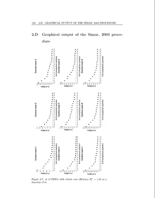
p.120: the following page merely contains a section title and a figure

\section{Graphical output of the Simar, 2003 procedure} 
\begin{minipage}{0.55\textheight}
\centering
\begin{adjustbox}{angle=90, center, caption=\# of DMUs with robust cost efficiency 
$\theta^{m}_{t}>$ 1.05 as a function of m, nofloat=figure} %,center
\includegraphics[width=1.7\linewidth]{Figures/simar1.05.png}  
\label{simarprocedure_single}
\end{adjustbox}
\end{minipage}
\FloatBarrier

Update: I set the heading over multiple lines as suggested by David Carlisle below. This gives the following code (output shown in the last printscreen). Now the table clearly fits within the page, but the problem remains?

\begin{sidewaystable}
\centering 
\caption{Set identification results for $\Omega$ based on LP-2 (sample size 500 obs)}
\label{MCboundsbeta}
%\resizebox{\textwidth}{!}{%
\setlength{\tabcolsep}{0.75\tabcolsep}
\begin{threeparttable}
\begin{tabular}{l|cc|cc|cc|cc}
\toprule
& \multicolumn{2}{c}{LP-1}
& \multicolumn{2}{c}{$\beta =$ 1} 
& \multicolumn{2}{c}{$\beta = $ .950} 
& \multicolumn{2}{c}{$\beta = $ .900} \\ \midrule
& $\# (\Omega^{true}$ 
& $\# (\Omega^{true}$ 
&  $\# (\Omega^{true}$ 
&  $\# (\Omega^{true}$ 
&  $\# (\Omega^{true}$ 
&  $\# (\Omega^{true}$ 
&  $\# (\Omega^{true}$ 
&  $\# (\Omega^{true}$ \\
& $>$ & $<$ & $>$ & $<$ & $>$ & $<$ &$>$ &$<$
\\
& $\Omega_{LP-OP})$ & $\Omega_{LP-OP})$ & $\Omega^{MIN}_{LP-2})$ & $\Omega^{MAX}_{LP-2})$ & $\Omega^{MIN}_{LP-2})$ & $\Omega^{MAX}_{LP-2})$ & $\Omega^{MIN}_{LP-2})$ & $\Omega^{MAX}_{LP-2})$
\\ \midrule
$\sigma^{2}_{\varepsilon}$=0    & 9.67 & 490.33  & 18.79  & 492.32 & 265.97    & 499.74  & 491.73 & 500 \\
$\sigma^{2}_{\varepsilon}$=.025 & 19.63 & 480.37 & 23.99 & 482.4 & 291.37 & 499.66 & 485.89  & 500 \\
$\sigma^{2}_{\varepsilon}$=.05  & 46.8 & 453.2 & 49.32  & 453.85 & 284.93 & 499.19 & 463.69  & 500 \\ \midrule
$\sigma^{2}_{\varepsilon}$=0   & (-) & (-) & 0 & 10  & 5.67  & 10     & 9.90 & 10  \\
$\sigma^{2}_{\varepsilon}$=.025 & (-) & (-)  & 0   & 10 & 6.44   & 10  & 9.96   & 10  \\
$\sigma^{2}_{\varepsilon}$=.05  & (-) & (-) & 0  & 10  & 6.15  & 10  & 9.73    & 10  \\ 
\bottomrule
\end{tabular}%
\begin{tablenotes}
\Large \item Note: Rows 1-3 show the frequency of correct set identification of $\Omega$ for individual observations. Similar results on the level of individual groups $i$ are reported in rows 4-6 (i.e. comparing the computed LP-2 objective function value with its true value). For the sample of 500 observations there are 10 such groups, each consisting of 50 observations.
\end{tablenotes}
\end{threeparttable}
%} %resizebox
\end{sidewaystable}

it is very hard to comment if you just post large blocks of code as fragments that can not be processed. It is much better to make a small complete test document that shows the problem. As a general rule it is better to avoid using resizebox on tables it forces inconsistent font sizes and rule widths — David Carlisle, Oct 11 '21 at 17:01
https://tex.stackexchange.com/questions/332902/my-table-doesnt-fit-what-are-my-options — David Carlisle, Oct 11 '21 at 17:02
the sideways table in your image has unreasonably wide columns as the headings are so much wider than the data. Set the heading over multiple lines, or truncate them in other ways. — David Carlisle, Oct 11 '21 at 17:03
The problem is the \includegraphics[width=1.7\linewidth]{...} is too big. \afterheading insures the \section goes with it. — John Kormylo, Oct 11 '21 at 20:52
Thanks for the answer! I tried setting the heading over multiple lines, yet the problem remains, even without resizebox. I made the following adjustment: & $# (\Omega^{true} > $ & $# (\Omega^{true} < $ & $# (\Omega^{true} > $ & $# (\Omega^{true} < $ & $# (\Omega^{true} > $ & $# (\Omega^{true} < $ & $# (\Omega^{true} > $ & $# (\Omega^{true} < $ \ & $\Omega_{LP-OP})$ & $\Omega_{LP-OP})$ & $\Omega^{MIN}{LP-2})$ & $\Omega^{MAX}{LP-2})$ & $\Omega^{MIN}{LP-2})$ & $\Omega^{MAX}{LP-2})$ & $\Omega^{MIN}{LP-2})$ & $\Omega^{MAX}{LP-2})$ The table is still too wide? — reteid94, Oct 12 '21 at 08:16
Moreover, using \setlength{\tabcolsep}{0.75\tabcolsep} to reduce horizontal separation (as suggested in the link you proposed) does not solve the issue. The table now clearly does not use up all the available page width or page length (without using resizebox) but the problem remains? I find it hard to believe that the table is still too wide? — reteid94, Oct 12 '21 at 08:26

John Kormylo · Answer 1 · 2021-10-13T13:37:44.380

Not sure where the 0.55\textheight comes from, but if that is the width you want:

\documentclass[10pt,twoside]{report}
\usepackage{appendix,amsmath,amscd,amssymb,amsfonts,amsthm,setspace,booktabs,pgfplotstable,a4wide,float,floatflt,bbm,tikz,pdflscape}
\usepackage{tikz,etoolbox,graphicx,chngpage,pdfpages,multirow,fancyhdr,verbatim,float,lscape,rotating,color, colortbl,longtable,graphicx,mathrsfs,eurosym,enumerate}
\usepackage[normalem]{ulem}
\usepackage[margin=1.75in]{geometry}
\usepackage{adjustbox}
\usepackage{refstyle}
\usepackage[colorlinks=true, citecolor=black, linkcolor=black, urlcolor=black,breaklinks]{hyperref}
\usepackage[round,authoryear]{natbib} 
\usepackage[flushleft]{threeparttable}
\usepackage[section]{placeins}
\usepackage{mathtools,subcaption,bm,arydshln,bookmark,chngcntr,titlesec}
\usetikzlibrary{positioning}
\newcommand{\npar}{\par \vspace{2.3ex plus 0.3ex minus 0.3ex}}
\setcounter{MaxMatrixCols}{10}
\newsavebox{\tempbox}
\begin{document}
\begin{sidewaystable}
\centering
\caption{Set identification results for $\Omega$ based on LP-2 (sample size 500 obs)}
\label{MCboundsbeta}
\resizebox{\textwidth}{!}{%
\begin{threeparttable}
\begin{tabular}{l|cc|cc|cc|cc}
\toprule
& \multicolumn{2}{c}{LP-1}
& \multicolumn{2}{c}{$\beta =$ 1} 
& \multicolumn{2}{c}{$\beta = $ .950} 
& \multicolumn{2}{c}{$\beta = $ .900} \ \midrule
& $# (\Omega^{true} > \Omega_{LP-OP})$ 
& $# (\Omega^{true} < \Omega_{LP-OP})$ 
&  $# (\Omega^{true} > \Omega^{MIN}{LP-2})$ 
&  $# (\Omega^{true} < \Omega^{MAX}{LP-2})$
&  $# (\Omega^{true} > \Omega^{MIN}{LP-2})$ 
&  $# (\Omega^{true} < \Omega^{MAX}{LP-2})$ 
&  $# (\Omega^{true} > \Omega^{MIN}{LP-2})$ 
&  $# (\Omega^{true} < \Omega^{MAX}{LP-2})$ 
\ \midrule
$\sigma^{2}{\varepsilon}$=0    & 9.67 & 490.33  & 18.79  & 492.32 & 265.97    & 499.74  & 491.73 & 500 \
$\sigma^{2}{\varepsilon}$=.025 & 19.63 & 480.37 & 23.99 & 482.4 & 291.37 & 499.66 & 485.89  & 500 \
$\sigma^{2}{\varepsilon}$=.05  & 46.8 & 453.2 & 49.32  & 453.85 & 284.93 & 499.19 & 463.69  & 500 \ \midrule
$\sigma^{2}{\varepsilon}$=0   & (-) & (-) & 0 & 10  & 5.67  & 10     & 9.90 & 10  \
$\sigma^{2}{\varepsilon}$=.025 & (-) & (-)  & 0   & 10 & 6.44   & 10  & 9.96   & 10  \
$\sigma^{2}{\varepsilon}$=.05  & (-) & (-) & 0  & 10  & 6.15  & 10  & 9.73    & 10  \ 
\bottomrule
\end{tabular}%
\begin{tablenotes}
\Large \item Note: Rows 1-3 show the frequency of correct set identification of $\Omega$ for individual observations. Similar results on the level of individual groups $i$ are reported in rows 4-6 (i.e. comparing the computed LP-2 objective function value with its true value). For the sample of 500 observations there are 10 such groups, each consisting of 50 observations.
\end{tablenotes}
\end{threeparttable}
} %resizebox
\end{sidewaystable}
\section{Graphical output of the Simar, 2003 procedure} 
\centering
\begin{minipage}{0.55\textheight}
\begin{adjustbox}{angle=90, center, caption=# of DMUs with robust cost efficiency 
$\theta^{m}_{t}>$ 1.05 as a function of m, nofloat=figure} %,center
\includegraphics[height=\linewidth]{example-image}
\label{simarprocedure_single}
\end{adjustbox}
\end{minipage}
\FloatBarrier
\end{document}

Now if you want to make the figure as large as possible and still fit the page:

Note that the caption may change height as the minipage shrinks, hence the loop.

\begingroup% use local registers
\setbox0=\vbox{\csname @minipagetrue\endcsname% if top of page
  \section{Graphical output of the Simar, 2003 procedure}}% measure height
\setlength{\dimen1}{\dimexpr \textheight-\ht0-\dp0}% rest of page, not including caption
\unvbox0
\dimen2=\textwidth
\loop
  \sbox1{\begin{minipage}{\dimen2}
    \vspace*{\abovecaptionskip}%
    \captionof{figure}{\# of DMUs with robust cost efficiency 
      $\theta^{m}_{t}>$ 1.05 as a function of m}
    \addtocounter{figure}{-1}%
   \end{minipage}}
  \sbox2{\includegraphics[height=\textwidth,width={\dimexpr \dimen1-\ht1-\dp1},keepaspectratio]{example-image-16x9}}%
  \ifdim\ht2<\dimen2
    \dimen2=\ht2
  \repeat
\refstepcounter{figure}\label{simarprocedure_single}%
\centering
\rotatebox{90}{\usebox2}\\
\noindent\usebox1\par
\endgroup

Thank you for your answer. It seems you made changes to the page 120. However, I think that the problem does not have to do with this page, as the empty page p.119 is classified under '2.C extensions' while the figure on p.120 is part of section 2.D? — reteid94, Oct 12 '21 at 08:14
No, the blank page has nothing to do with the sidewaysfigure, or anything before the\section{Graphical...}. — John Kormylo, Oct 12 '21 at 13:51
You are indeed correct, once I remove p.120 the problem no longer appears. However, when copying your suggestions, the blank page does not disappear. However, the problem resolved after setting \includegraphics[height=0.8\linewidth]. Thank you for your help! — reteid94, Oct 13 '21 at 07:37

How to remove empty page created by sidewaystable in a threeparttable with resizebox (shrinking table does not work)?

1 Answers1