Trying to plot y^2 = x^3 + 5 (tikz)

Question

I'm trying to plot an elliptic curve but it leaves a weird "gap". I have tried different values for the domain but the gap remains.

    \begin{tikzpicture}
        \begin{axis}[
            xmin=-2.5,
            xmax=3,
            ymin=-5,
            ymax=5,
            xlabel={$x$},
            ylabel={$y$},
            scale only axis,
            axis lines=middle,
            domain=-1.71:3,
            samples=200,
            smooth,
            % to avoid that the "plot node" is clipped (partially)
            clip=false,
            % use same unit vectors on the axis
            axis equal image=true,
        ]
            \addplot [red] {sqrt(x^3+5)};
            \addplot [red] {-sqrt(x^3+5)};
    \end{axis}

\end{tikzpicture}

Just change the domain to domain=-1.709975:3 – Sandy G Mar 30 '22 at 15:23 — Sandy G, Mar 30 '22 at 15:23

score 13 · Answer 1 · edited Apr 05 '22 at 17:34

You get

NOTE: coordinate (2Y1.71e0],3Y0.0e0]) has been dropped because it is unbounded
(in y). (see also unbounded coords=jump).
NOTE: coordinate (2Y1.71e0],3Y0.0e0]) has been dropped because it is unbounded
(in y). (see also unbounded coords=jump).

Compute the cube root of 5 like TikZ would.

\documentclass{article}
\usepackage{pgfplots}
\pgfplotsset{compat=1.18}
\begin{document}
\begin{tikzpicture}
  \pgfmathsetmacro{\cuberootoffive}{exp(ln(5)/3)}
  \begin{axis}[
    xmin=-2.5,
    xmax=3,
    ymin=-5,
    ymax=5,
    xlabel={$x$},
    ylabel={$y$},
    scale only axis,
    axis lines=middle,
    domain=-\cuberootoffive:3,
    samples=200,
    smooth,
    % to avoid that the "plot node" is clipped (partially)
    clip=false,
    % use same unit vectors on the axis
    axis equal image=true,
  ]
    \addplot [red] {sqrt(x^3+5)};
    \addplot [red] {-sqrt(x^3+5)};
  \end{axis}
\end{tikzpicture}
\end{document}

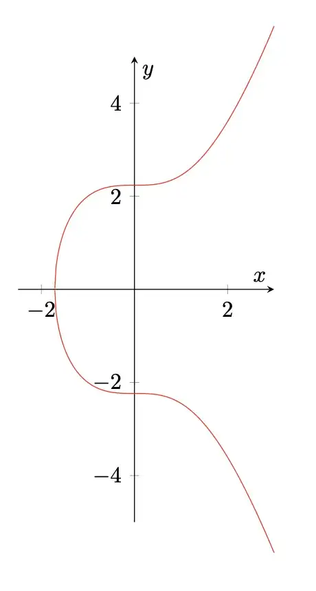
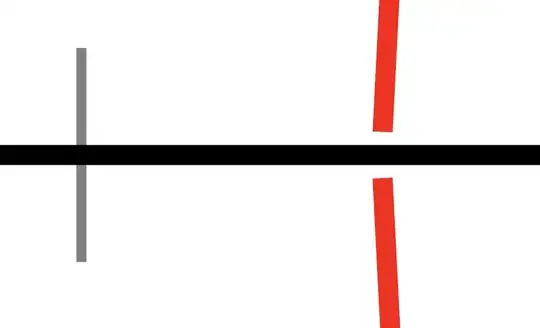
There is still a tiny gap, though:

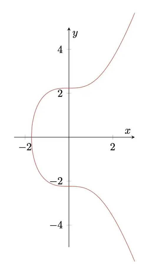
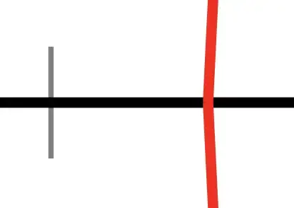
No gap with xfp and the graph is actually correct.

\documentclass{article}
\usepackage{pgfplots}
\usepackage{pgfmath-xfp,xfp}
\pgfplotsset{compat=1.18}
\begin{document}
\begin{tikzpicture}
  \edef\cuberootoffive{\fpeval{exp(ln(5)/3)}}
  \pgfmxfpdeclarefunction{cubic}{1}{sqrt((#1)^3+5)}
  \begin{axis}[
    xmin=-2.5,
    xmax=3,
    ymin=-5,
    ymax=5,
    xlabel={$x$},
    ylabel={$y$},
    scale only axis,
    axis lines=middle,
    domain=-\cuberootoffive:3,
    samples=200,
    smooth,
    % to avoid that the "plot node" is clipped (partially)
    clip=false,
    % use same unit vectors on the axis
    axis equal image=true,
  ]
    \addplot [red] {cubic(x)};
    \addplot [red] {-cubic(x)};
  \end{axis}
\end{tikzpicture}
\end{document}

+1: Is the xfp package "only" needed for the domain calculation? — Dr. Manuel Kuehner, Apr 05 '22 at 17:33
@Dr.ManuelKuehner Yes. But in a short time it will no longer be needed. — egreg, Apr 05 '22 at 17:34
Ok, I saw the message "From 2022-06-01 release of LATEX this will be included in the format so that the package doesn't need loading any longer." — Dr. Manuel Kuehner, Apr 05 '22 at 17:35
Hm, compile time takes quite a hit from using xfp. On average 883.1 ms for xfp vs. 627.6 ms for pgfmath. — Henri Menke, Apr 05 '22 at 17:44
@HenriMenke That's true. But what about getting the right output instead of a faulty one? :-) — egreg, Apr 05 '22 at 17:45
@egreg Plots requiring high accuracy should just not be done in TeX in the first place. I used to plot everything in TeX as well, but at some point got tired of compile times of the order of 5 minutes and just switch to gnuplot. — Henri Menke, Apr 05 '22 at 17:48

score 10 · Answer 2 · answered Mar 30 '22 at 20:13

You can plot implicit functions curves with the pstricks package pst-func. Here is a code for that:

    \documentclass[svgnames, pstricks, border=10pt]{standalone}
    \usepackage{pst-plot,pst-func }
\begin{document}

\begin{pspicture*}(-3,-5)(3,5)
\psset{plotpoints=4000, showorigin=false, arrowinset=0.12, linejoin=1}
\psaxes[labelFontSize=\scriptstyle,ticksize=0 4pt, Dx=2, Dy=2]{-&gt;}(0,0)(-3,-5)(3,5)[$x$,-120][$y$,210]
\psplotImp[algebraic, linecolor=Tomato, linewidth=1.2pt](-4,-6)(4,6){x^3-y^2 + 5}
\end{pspicture*}

\end{document}

Black Mild · Answer 3 · 2022-03-31T06:28:13.997

Here is an Asymptote drawing for that implicit function. Also see this answer.

// Run on http://asymptote.ualberta.ca/
unitsize(1cm);
import contour;
import graph;
real f(real x, real y) { return y^2-x^3; }
pair A=(-2.5,-5), B=(3,5);
limits(A,B);
guide[][] g = contour(f,A,B, new real[] {5});
draw(g[0],blue+1pt);
real[] x={-2,2};
real[] y={-4,-2,2,4};
xaxis(Label("$x$",EndPoint,align=N),Ticks(x,1mm,red));
yaxis(Label("$y$",EndPoint,align=E),Ticks(y,1mm,red));
shipout(bbox(5mm,invisible));

score 4 · Answer 4 · answered Mar 31 '22 at 05:11

As pgfplots cannot (as far as I can see?) plot implicit curve, you have to manually parametrize it _{(or switch to another package like explained in the other answer)}, and if you want good curve you have to find good parametrization.

In this case, let the parameter be the variable y works better:

%! TEX program = lualatex
\documentclass{article}
\usepackage{pgfplots}
\pgfplotsset{compat=1.12}
\begin{document}
\begin{tikzpicture}
\begin{axis}[
    xmin=-2.5,
    xmax=3,
    ymin=-5,
    ymax=5,
    xlabel={$x$},
    ylabel={$y$},
    scale only axis,
    axis lines=middle,
    smooth,
    % to avoid that the "plot node" is clipped (partially)
    clip=false,
    % use same unit vectors on the axis
    axis equal image=true
    ]
\addplot [variable=t, domain=-5:5, samples=50, red] ({abs(t^2-5)^0.333333333333*sign(t^2-5)}, {t});
\end{axis}
\end{tikzpicture}
\end{document}

Reference: https://tex.stackexchange.com/a/582731/250119 (manual parametrization example) How can I draw an implicit equation with pgfplots? (how to cube root) Using pgfplots to create 2-D parameterized parametric plot (how to plot parametrized)

Trying to plot y^2 = x^3 + 5 (tikz)

4 Answers4

Linked