How to draw a shaded boundary using TikZ

Question

How can I draw a simple shaded region such as the one shown below using TikZ?

The shaded region bounded by the equation

r1r2r3 - r1 - r2 - r3 + 2cos(theta)

and is r1=r2=r3=4. The boundary will change slightly for different values of theta. For the purpose of this, we can assume theta=0.

The idea here is to use TikZ with certain functions and fillbetween commands but this becomes tricky for 3D plots. This example could then be used to draw more involved boundaries

Any tips/relevant posts would be helpful!

EDIT

I would ideally like a solution that just uses TiKZ and not pstricks.

What is your figure? A lot of details should be added, in my opinion — Black Mild, May 08 '22 at 04:49
@BlackMild, thank you for the suggestion. Please see updated question. — Sid, May 08 '22 at 09:52
What about using some faster programming language to generate list of coordinates then feed that one to TikZ instead? (that would probably also be faster. — user202729, May 08 '22 at 11:10
@user202729, that would be the go-to method if this fails. Ideally, I would like to learn how to approach this via TikZ alone — Sid, May 08 '22 at 11:27
Well if I recalled correctly TikZ does not have a "real" 3D engine, so first step would be to let the viewpoint be (x, y, z) (given the image I assume you want perspective projection instead of central projection, as the bottom face is much larger than the top face in the projection), hope that the formula is simple/can be expressed in elementary functions, etc. — user202729, May 08 '22 at 11:32
Doesn't sound fun. Plugging in something with a 3D engine sounds like less work. — user202729, May 08 '22 at 11:33
Anyway do you require central/perspective projection, or is parallel (orthographic) projection okay? — user202729, May 08 '22 at 11:40
A 2D projection may obscure some of the details, particularly when looking for a solution that can be extended to more involved boundaries, so a central/perspective would be more suited. — Sid, May 08 '22 at 11:52
Related question, there is pgfplots - plot 3d graphs of functions defined implicitly - TeX - LaTeX Stack Exchange for plotting implicit 3d surface, but I'm not sure if the engine support transparency. There's also tikz pgf - Drawing intersecting 3D surface plots - TeX - LaTeX Stack Exchange for transparent, but it's for pstricks — user202729, May 08 '22 at 23:36

score 2 · Answer 1 · answered May 26 '22 at 09:53

I think that implicit surfaces can be sketched in TikZ when the level curves (or other hyperplane sections) can be drawn. For the surface xyz - x - y - z + 2 = 0 (in fact for any value of theta in the question), the level curves are hyperbolas and it is not difficult to draw them.

Some comments

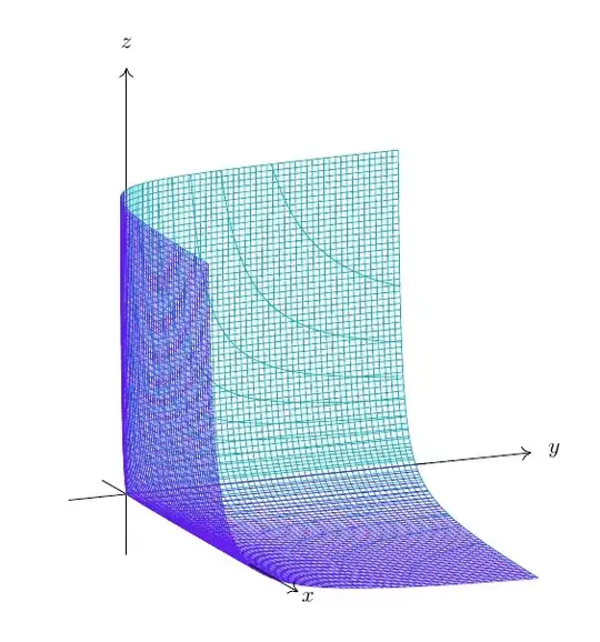
I changed the coordinates as to have the singular point at the origin, i.e. I considered the surface defined by xyz + xy + yz + zx = 0. It is only a translation of the previous one.
Looking at the example that it was given, I represented only a "sheet" of the surface; explicitly I considered the portion of the surface living in the cube [-1, 5]^3 and which is swept out by only one branch of each z=h hyperbola.
For z=0 the hyperbola degenerates into the union of two lines. For z=-1 it degenerates again into two lines, but one is at infinity. For these reasons, the drawing of the level curve depends on the sign of z. In the neighborhood of -1 things are more subtle since the limits of TikZ are easily reached. For example, if the first \foreach is performed for \i=1 or \i=2, the curves obtained are not "real" (or at least the intended ones).
The code might seem long, but what counts are the first two \foreach commands that draw the z=h level curves. Afterwards, they are just copied and modified in order to obtain the x=h and y=h level curves.
Each branch of a hyperbola is drawn as a parametrized curve; the bounds of the parameter are computed to obtain only the portion inside the cube.

The code

\documentclass[margin=.5cm]{standalone}
\usepackage{tikz}
\usetikzlibrary{math}
\usepackage{tikz-3dplot}
\usetikzlibrary{3d}
\usetikzlibrary{arrows.meta}
\begin{document}
\xdefinecolor{Cy}{RGB}{17, 170, 187}
\xdefinecolor{VB}{RGB}{102, 25, 240}
\tikzmath{
  integer \N-, \N+;
  \N- = 12;
  \N+ = 50;
  real \a;
  \a = 5;
}
\tikzset{
  pics/level curve+/.style args={height=#1, varbound=#2, color=#3}{%
    code={%
      \draw[#3, variable=\t, domain=-#2:#2, samples=40]
      plot ({#1/(#1 +1)(exp(\t) -1)}, {#1/(#1 +1)(exp(-\t) -1)});
    }
  },
  pics/level curve-/.style args={height=#1, varbound=#2, color=#3}{%
    code={%
      \draw[#3, variable=\t, domain=-#2:#2, samples=40]
      plot ({-#1/(#1 +1)(exp(\t) +1)}, {-#1/(#1 +1)(exp(-\t) +1)});
    }
  }
}
\begin{tikzpicture}
  \tdplotsetmaincoords{76}{67}
  \begin{scope}[tdplot_main_coords]
    % axes first part
    \draw (-1, 0, 0) -- (\a +.2, 0, 0);
    \draw (0, -1, 0) -- (0, \a +.2, 0);
    \draw (0, 0, -1) -- (0, 0, \a +.2);
%%% $z=h$ level curves
% close to $0^-$
\foreach \i
[evaluate=\i as \h using {-(\N- +1 -\i)/(\N- +1))*\a/(\a +1)},
evaluate=\i as \b using {ln(-(\h +1)*\a/\h -1)}]
in {1, 2, 3, 4, ..., \N-}{
  \path[canvas is xy plane at z=\h, transform shape] (0, 0)
  pic {level curve-={height=\h, varbound=\b, color=Cy}};
}    

% $h=0$
\draw[Cy, canvas is xy plane at z=0] (0, \a) |- (\a, 0);

% $h&gt;0$
\foreach \i
[evaluate=\i as \h using {(\i/\N+)*\a},
evaluate=\i as \b using {ln((\h +1)*\a/\h +1)}]
in {1, 2, ..., \N+}{
  \path[canvas is xy plane at z=\h, transform shape] (0, 0)
  pic {level curve+={height=\h, varbound=\b, color=Cy}};
}

%%% $y=h$ level curves
% close to $0^-$
\foreach \i
[evaluate=\i as \h using {-(\N- +1 -\i)/(\N- +1))*\a/(\a +1)},
evaluate=\i as \b using {ln(-(\h +1)*\a/\h -1)}]
in {3, 4, ..., \N-}{
  \path[canvas is xz plane at y=\h, transform shape] (0, 0)
  pic {level curve-={height=\h, varbound=\b, color=Cy}};
}    

% $h=0$
\draw[Cy, thin, canvas is xz plane at y=0] (0, \a) |- (\a, 0);

% $h&gt;0$
\foreach \i
[evaluate=\i as \h using {(\i/\N+)*\a},
evaluate=\i as \b using {ln((\h +1)*\a/\h +1)}]
in {1, 2, ..., \N+}{
  \path[canvas is xz plane at y=\h, transform shape] (0, 0)
  pic {level curve+={height=\h, varbound=\b, color=Cy}};
}

%%% $x=h$ level curves
% close to $0^-$
\foreach \i
[evaluate=\i as \h using {-(\N- +1 -\i)/(\N- +1))*\a/(\a +1)},
evaluate=\i as \b using {ln(-(\h +1)*\a/\h -1)}]
in {3, 4, ..., \N-}{
  \path[canvas is yz plane at x=\h, transform shape] (0, 0)
  pic {level curve-={height=\h, varbound=\b, color=Cy}};
}    

% $h=0$
\draw[VB, canvas is yz plane at x=0] (0, \a) |- (\a, 0);

% $h&gt;0$
\foreach \i
[evaluate=\i as \h using {(\i/\N+)*\a},
evaluate=\i as \b using {ln((\h +1)*\a/\h +1)}]
in {1, 2, ..., \N+}{
  \path[canvas is yz plane at x=\h, transform shape] (0, 0)
  pic {level curve+={height=\h, varbound=\b, color=VB}};
}

%%% axes second part
\begin{scope}[arrows={-&gt;[length=1ex, width=1.5ex]}]
  \draw (\a, 0, 0) -- (\a +2, 0, 0)  node[pos=1.2] {$x$};
  \draw (0, \a, 0) -- (0, \a +2, 0)  node[pos=1.2] {$y$};
  \draw (0, 0, \a) -- (0, 0, \a +2)  node[pos=1.2] {$z$};          
\end{scope}

\end{scope}
\end{tikzpicture}
\end{document}

How to draw a shaded boundary using TikZ

1 Answers1